Why Study Probability?

Probability is the science of uncertainty, empowering you to make informed decisions in data science and everyday life. It’s essential because:

  • Data Science: Drives machine learning (e.g., spam filters), statistical modeling, and predictive analytics (e.g., customer behavior).
  • Real Life: Informs weather forecasts, medical diagnoses, financial investments, and game strategies.
  • Critical Thinking: Equips you to calculate chances, assess risks, and interpret data accurately.

Probability Basics

Key Definitions

Probability measures how likely an event is. Here are the core concepts:

  • Probability (\(P(A)\)):
    • Definition: Chance of event \(A\) happening, ranging from 0 to 1.
    • Formula: \(P(A) = \frac{|A|}{|\Omega|}\) = \(\frac{\text{Favorable outcomes}}{\text{Total outcomes}}\).
    • Example: \(P(\text{Rolling a 6}) = \frac{1}{6}\).
  • Experiment:
    • Definition: An action with uncertain results.
    • Example: Flipping a coin.
  • Outcome:
    • Definition: One possible result of an experiment.
    • Example: Getting Heads.
  • Sample Space (\(\Omega\) or \(S\)):
    • Definition: Set of all possible outcomes.
    • Notation: \(\Omega = \{x_1, x_2, \ldots\}\).
    • Example: For a coin flip, \(\Omega = \{\text{Heads}, \text{Tails}\}\).
  • Event (\(A \subseteq \Omega\)):
    • Definition: A subset of outcomes from the sample space.
    • Example: \(A = \{\text{Heads}\}\) for getting Heads.
  • Sure Event (\(\Omega\)):
    • Definition: Includes all outcomes; always happens.
    • Formula: \(P(\Omega) = 1\).
    • Example: Rolling a number 1–6 on a die.
  • Impossible Event (\(\emptyset\)):
    • Definition: Includes no outcomes; never happens.
    • Formula: \(P(\emptyset) = 0\).
    • Example: Rolling a 7 on a die.
  • Random Variable (\(X\)):
    • Definition: A number assigned to each outcome.
    • Notation: \(X: \Omega \to \mathbb{R}\).
    • Example: \(X\) = Number of Heads in two coin flips (\(0\), \(1\), \(2\)).
  • Probability Line:
0 (Impossible) ---- Possible ---- 1 (Sure)

Sample Space Examples

The sample space \(\Omega\) lists all outcomes. For an experiment with sample space \(\Omega\) repeated \(n\) times independently, the sample space is \(\Omega^n\) (Cartesian product), with size \(|\Omega|^n\).

  • Rolling a die once:
    • \(\Omega = \{1, 2, 3, 4, 5, 6\}\), \(|\Omega| = 6\).
    • Event: \(A = \{2, 4, 6\}\) (even numbers).
  • Flipping a coin twice:
    • \(\Omega = \{\text{H}, \text{T}\}\), \(\Omega^2 = \{\text{HH}, \text{HT}, \text{TH}, \text{TT}\}\), \(|\Omega|^2 = 2^2 = 4\).
    • Event: \(A = \{\text{HT}, \text{TH}\}\) (exactly one Head).
  • Counting Heads in three coin flips:
    • \(\Omega = \{\text{HHH}, \text{HHT}, \ldots, \text{TTT}\}\), \(|\Omega| = 2^3 = 8\).
    • Random variable \(X\): Number of Heads, \(\Omega_X = \{0, 1, 2, 3\}\).
  • Rolling two dice:
    • \(\Omega = \{(i, j) \mid i, j = 1, \ldots, 6\}\), \(|\Omega| = 6^2 = 36\).

Understanding Events

Types of Events

Events describe possible outcomes in \(\Omega\).

  • Mutually Exclusive Events: Cannot occur together.
    • Notation: \(A \cap B = \emptyset\).
    • Formula: \(P(A \cup B) = P(A) + P(B)\).
    • Example: Rolling a 3 or 4 on a die.
  • Independent Events: One doesn’t affect the other.
    • Notation: \(P(A \cap B) = P(A) \cdot P(B)\).
    • Formula: \(P(A \text{ given } B) = P(A | B) = P(A)\).
    • Example: Flipping Heads and rolling a 6.
  • Sure Event: Includes all outcomes.
    • Notation: \(A = \Omega\), \(P(\Omega) = 1\).
    • Example: Die shows a number.
  • Impossible Event: Includes no outcomes.
    • Notation: \(A = \emptyset\), \(P(\emptyset) = 0\).
    • Example: Die shows a letter.

Common Pitfall: Mutually exclusive (no overlap) differs from independent (no influence). Coin flip and die roll are independent, not mutually exclusive.

Example:

  • Mutually Exclusive: Picking a red or blue ball.
  • Independent: Rain and forgetting your umbrella.

Question: Are “drawing an Ace” and “drawing a King” mutually exclusive? Independent?

Set Theory for Probability

Sets and Operations

Events are sets in \(\Omega\), visualized with Venn diagrams.

  • Union: \(A \cup B\) = Outcomes in \(A\), \(B\), or both.
    • Formula: \(P(A \cup B) = P(A) + P(B) - P(A \cap B)\).
  • Intersection: \(A \cap B\) = Outcomes in both \(A\) and \(B\).
    • Formula: \(P(A \cap B) = P(A) \cdot P(B \text{ given } A)\).
  • Complement: \(A' = \Omega \setminus A\) = Outcomes not in \(A\).
    • Formula: \(P(A') = 1 - P(A)\).

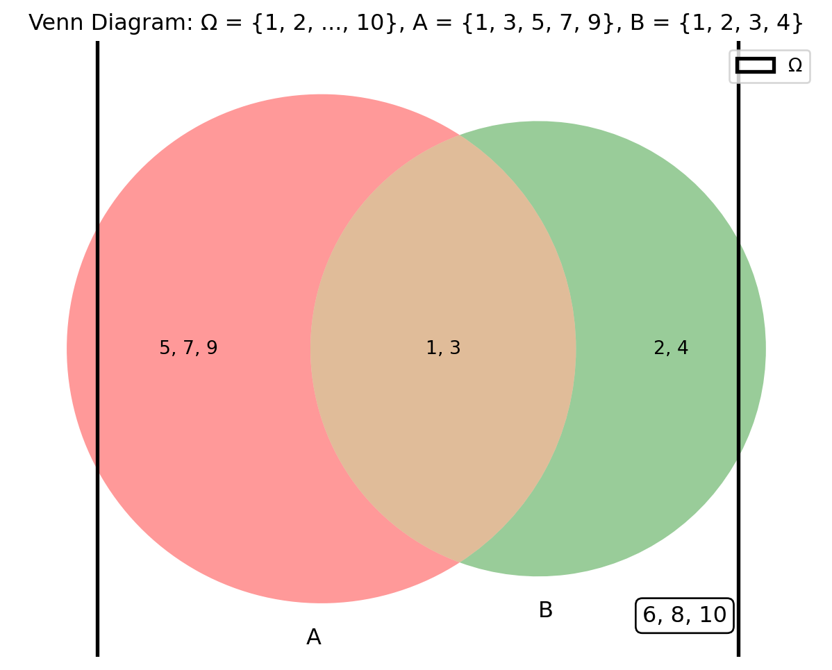
Example: \(\Omega = \{1, 2, \ldots, 10\}\), \(A = \{1, 3, 5, 7, 9\}\), \(B = \{1, 2, 3, 4\}\).

  • \(A \cup B = \{1, 2, 3, 4, 5, 7, 9\}\).
  • \(A \cap B = \{1, 3\}\).
  • \(A' = \{2, 4, 6, 8, 10\}\).

Venn Diagram: Visualizing sets \(A\) and \(B\) in \(\\Omega\)

Probability Rules

Simple Rules to Calculate Chances

  • Basic Rule:
    • \(P(A) = \frac{\text{Number of outcomes in } A}{\text{Total outcomes in } \Omega} = \frac{|A|}{|\Omega|}\).
    • Example: \(P(\text{Rolling a 6}) = \frac{1}{6}\).
  • Addition Rule:
    • Any events: \(P(A \cup B) = P(A) + P(B) - P(A \cap B)\).
    • Mutually exclusive: \(P(A \cup B) = P(A) + P(B)\).
  • Multiplication Rule:
    • Independent: \(P(A \cap B) = P(A) \cdot P(B)\).
    • Dependent: \(P(A \cap B) = P(A) \cdot P(B \text{ given } A)\).
  • Complement Rule:
    • \(P(A') = 1 - P(A)\).
    • Example: \(P(\text{Not 6}) = 1 - \frac{1}{6} = \frac{5}{6}\).
  • Total Probability:
    • For mutually exclusive, exhaustive events \(A_1, \ldots, A_n\):
      • \(P(B) = \sum_{i=1}^n P(B | A_i) \cdot P(A_i)\).

Example: Bag with 2 red, 3 blue balls:

  • \(P(\text{Red}) = \frac{2}{5}\), \(P(\text{Blue}) = \frac{3}{5}\).
  • \(P(\text{Red or Blue}) = \frac{2}{5} + \frac{3}{5} = 1\) (mutually exclusive).

Tip: Check for overlap in “or” problems to avoid double-counting.

Exercise: If \(P(A) = 0.5\), \(P(B) = 0.4\), and \(A \cap B = \emptyset\), find \(P(A \cup B)\).

Conditional Probability: What Happens If…?

Chance of \(A\) given \(B\) has occurred:

  • Formula: \(P(A | B) = \frac{P(A \cap B)}{P(B)}\), where \(P(B) > 0\).
  • Example: Drawing two aces without replacement.
    • \(P(1^\text{st} \text{Ace}) = \frac{4}{52}\).
    • \(P(2^\text{nd} \text{Ace} | 1^\text{st} \text{Ace}) = \frac{3}{51}\).
    • \(P(\text{Both Aces}) = \frac{4}{52} \cdot \frac{3}{51} \approx 0.0045\).

Bayes’ Theorem: Flipping the Question

Bayes’ Theorem: Find \(P(A| B)\) using \(P(B | A)\).

  • Formula: \(P(A | B) = \frac{P(B | A) \cdot P(A)}{P(B)}\).
  • Total Probability: \(P(B) = \sum_{i} P(B | A_i) \cdot P(A_i)\) for partitions \(A_i\).

Example: Pregnancy test (Exercise #1)

  • \(P(\text{Pregnant}) = 0.1\), \(P(\text{Positive | Pregnant}) = 0.98\).
  • Bayes’ finds: \(P(\text{Pregnant | Positive})\).
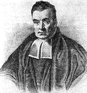
Thomas Bayes | 1701 – 1761 | English statistician and philosopher

Expected Value and Variance

Predicting Outcomes

  • Expected Value: Average outcome of random variable \(X\).
    • Formula: \(E[X] = \sum_x x \cdot P(X = x)\).
    • Example: Expected heads in two coin tosses:
      • \(E[X] = 0 \cdot \frac{1}{4} + 1 \cdot \frac{1}{2} + 2 \cdot \frac{1}{4} = 1\).
  • Variance: Measures spread of outcomes.
    • Formula: \(\text{Var}(X) = \sum_x (x - E[X])^2 \cdot P(X = x)\).
    • Example: Variance for two tosses = 0.5.
  • Standard Deviation: \(\text{SD}(X) = \sqrt{\text{Var}(X)}\).

Example Table:

\(x\) (Heads) \(P(X = x)\) \(x \cdot P(X = x)\)
0 1/4 0
1 1/2 0.5
2 1/4 0.5
Total 1 1

Exercise: Find \(E[X]\) for number of red balls in Exercise #3.

Counting Techniques

Introduction to Counting

Counting outcomes determines the size of \(\Omega\) and \(A\) in \(P(A) = \frac{|A|}{|\Omega|}\). Key principles include:

  • Multiplication Principle: If one event has \(m\) outcomes and another has \(n\), the combined event has \(m \cdot n\) outcomes.
    • Formula: For \(k\) independent stages with \(n_1, n_2, \ldots, n_k\) choices, total outcomes = \(n_1 \cdot n_2 \cdot \ldots \cdot n_k\).
    • Intuition: Each choice multiplies possibilities, like branches on a tree.
    • Example: Choosing a shirt (3 colors) and pants (2 styles):
      • Total outfits = \(3 \cdot 2 = 6\).
  • Addition Principle: For mutually exclusive events, total outcomes are the sum.
    • Formula: If event \(A\) has \(|A|\) outcomes and \(B\) has \(|B|\) with \(A \cap B = \emptyset\), total = \(|A| + |B|\).
    • Intuition: Add possibilities that cannot happen together.
    • Example: Choosing a fruit (3 apples) or a vegetable (2 carrots):
      • Total choices = \(3 + 2 = 5\).

Permutations: Arranging Items

Permutations count ways to arrange \(k\) distinct items from \(n\), where order matters.

  • Formula: \(P(n, k) = \frac{n!}{(n-k)!}\), where \(n! = n \cdot (n-1) \cdot \ldots \cdot 1\).
  • Intuition: Arrange items in specific positions, like seating people in a row.
  • Example 1: Arrange 3 letters (A, B, C) in 2 positions.
    • \(P(3, 2) = \frac{3!}{(3-2)!} = \frac{6}{1} = 6\).
    • Outcomes: AB, BA, AC, CA, BC, CB.
  • Example 2: Arrange 5 people in 3 chairs.
    • \(P(5, 3) = \frac{5!}{(5-3)!} = \frac{120}{2} = 60\).
  • With Repetition: If items can be repeated, use \(n^k\).
    • Example: 3-digit codes from digits 0–9 = \(10^3 = 1000\).

Tip: Use permutations for ordered arrangements (e.g., race rankings).

Combinations: Choosing Items

Combinations count ways to choose \(k\) distinct items from \(n\), where order does not matter.

  • Formula: \(\binom{n}{k} = \frac{n!}{k!(n-k)!}\).
  • Intuition: Pick items without caring about order, like forming teams.
  • Example 1: Choose 2 fruits from {Apple, Banana, Orange}.
    • \(\binom{3}{2} = \frac{3!}{2!1!} = \frac{6}{2 \cdot 1} = 3\).
    • Outcomes: {Apple, Banana}, {Apple, Orange}, {Banana, Orange}.
  • Example 2: Choose 3 students from 5 for a committee.
    • \(\binom{5}{3} = \frac{5!}{3!2!} = \frac{120}{6 \cdot 2} = 10\).
  • Connection to Probability: In Exercise #2, \(P(\text{Both Green}) = \frac{\binom{2}{2}}{\binom{9}{2}}\).

Advanced Counting Techniques

  • Permutations with Indistinguishable Objects:
    • Formula: For \(n\) items with groups of \(n_1, n_2, \ldots\) identical items, arrangements = \(\frac{n!}{n_1! n_2! \ldots}\).
    • Example: Arrange letters in MISS (\(2\) S’s, \(1\) M, \(1\) I).
      • \(\frac{4!}{2!1!1!} = \frac{24}{2} = 12\).
  • Combinations with Repetition:
    • Formula: Choose \(k\) items from \(n\) types with repetition = \(\binom{n+k-1}{k}\).
    • Example: Choose 2 fruits (Apple, Banana) with repetition.
      • \(\binom{2+2-1}{2} = \binom{3}{2} = 3\).
      • {Apple, Apple}, {Apple, Banana}, {Banana, Banana}.

Which Counting Technique to Use?

Technique Scenario/Case Key Questions Formula Example
Multiplication Principle Sequential, independent choices. Are there multiple stages? Can choices repeat? \(n_1 \cdot n_2 \cdot \ldots \cdot n_k\) Shirt (3) and pants (2): \(3 \cdot 2 = 6\).
Addition Principle Mutually exclusive choices. Are options exclusive? No overlap? \(|A| + |B|\) Apples (3) or carrots (2): \(3 + 2 = 5\).
Permutations Ordered arrangements of distinct items. Does order matter? Are items unique? \(P(n, k) = \frac{n!}{(n-k)!}\) Arrange 3 letters in 2 spots: \(P(3, 2) = 6\).
Combinations Unordered selections of distinct items. Does order not matter? Are items unique? \(\binom{n}{k} = \frac{n!}{k!(n-k)!}\) Choose 2 fruits from 3: \(\binom{3}{2} = 3\).
Permutations with Repetition Ordered arrangements, items can repeat. Can items repeat? Are choices independent? \(n^k\) 3-digit codes (0–9): \(10^3 = 1000\).
Indistinguishable Objects Arrange items with some identical. Are some items identical? \(\frac{n!}{n_1! n_2! \ldots}\) Arrange “MISS”: \(\frac{4!}{2!1!1!} = 12\).
Combinations with Repetition Unordered selections with repetition allowed. Can items repeat? Order doesn’t matter? \(\binom{n+k-1}{k}\) 2 fruits (Apple, Banana): \(\binom{3}{2} = 3\).

Tip: Ask “Does order matter?” and “Can items repeat?” to start.

Counting in Probability

Counting determines \(|\Omega|\) and \(|A|\) for \(P(A) = \frac{|A|}{|\Omega|}\).

  • Example: Probability of drawing 2 green marbles (Exercise #2).
    • \(\Omega\): All 2-marble combinations, \(\binom{9}{2} = 36\).
    • \(A\): 2 green marbles, \(\binom{2}{2} = 1\).
    • \(P(\text{2 green}) = \frac{1}{36}\).
  • Repeated Experiments: Use \(|\Omega|^n\).
    • Example: 3 coin flips, \(|\Omega| = 2^3 = 8\), \(P(\text{3 Heads}) = \frac{1}{8}\).

Why It Matters: Accurate counting ensures correct probabilities.

Exercise: Calculate \(P(4, 2)\) and \(\binom{4}{2}\). How do they differ in a probability context?

Probability Exercises

Exercise #1

If a woman takes an early pregnancy test, she will either test positive, meaning that the test says she is pregnant, or test negative, meaning that the test says she is not pregnant. Suppose that if a woman really is pregnant, there is a 98% chance that she will test positive. Also suppose that if a woman really is not pregnant, there is a 99% chance that she will test negative.

Pregnancy Test
  1. Suppose that 1,000 woman take early pregnancy tests and that 100 of them truly pregnant. What is the probability that a randomly chosen woman from this group will test positive?

  2. Suppose a woman tests positive. What is the probability that she really is pregnant?

Overview

This analysis uses a sample of 1,000 women undergoing early pregnancy tests, with the following assumptions:

  • If a woman is truly pregnant, the test is positive 98% of the time.
  • If a woman is not pregnant, the test is negative 99% of the time.

Total Population:

  • 1,000 women, with 100 truly pregnant (10%) and 900 not pregnant (90%).

Probability Calculations:

  1. Probability of a Positive Test (Overall) \[ P(\text{Test Positive}) = P(\text{Test Positive | Pregnant}) \times P(\text{Pregnant}) + P(\text{Test Positive | Not Pregnant}) \times P(\text{Not Pregnant}) \]

\[ = 0.98 \times 0.1 + 0.01 \times 0.9 = 0.107 \] - Result: 10.7% chance of testing positive across all 1,000 women.

  1. Probability of Being Pregnant Given a Positive Test

\[ P(\text{Pregnant | Test Positive}) = \frac{P(\text{Test Positive | Pregnant}) \times P(\text{Pregnant})}{P(\text{Test Positive})} \]

\[ = \frac{0.98 \times 0.1}{0.107} \approx 0.916 \] - Result: 91.6% chance of being pregnant if tested positive.

Tree Diagram for Probability Calculation

This diagram illustrates the probability pathways based on pregnancy status and test outcomes:

graph TD;
    A[Start: 1,000 Women] -->|10% Pregnant| B[Pregnant]
    A -->|90% Not Pregnant| C[Not Pregnant]
    B -->|98% Test Positive| D[Test Positive]
    B -->|2% Test Negative| E[Test Negative]
    C -->|1% Test Positive| F[Test Positive]
    C -->|99% Test Negative| G[Test Negative]

    style D fill:#4daf4a,color:#ffff
    style E fill:#e41a1c,color:#ffff
    style F fill:#4daf4a,color:#ffff
    style G fill:#4daf4a,color:#ffff

Exercise #2

A box contains 3 blue, 2 green, and 4 red marbles. If you draw 2 marbles at random without replacement, what is the probability both are green?

Probability Calculation: Drawing Two Green Marbles

Given a box with 3 blue, 2 green, and 4 red marbles, we are asked to find the probability of drawing two green marbles when drawing two marbles at random without replacement. Here’s the step-by-step calculation:

Total Number of Marbles

  • Blue Marbles: 3
  • Green Marbles: 2
  • Red Marbles: 4
  • Total: 3 + 2 + 4 = 9 marbles

Total Ways to Draw 2 Marbles from 9

Using the combination formula \(\binom{n}{k}\) which represents the number of ways to choose \(k\) items from \(n\) items without regard to the order, we calculate:

\[ \binom{9}{2} = \frac{9 \times 8}{2 \times 1} = 36 \]

Ways to Draw 2 Green Marbles from 2 Available

There are 2 green marbles and we need to draw both:

\[ \binom{2}{2} = \frac{2 \times 1}{2 \times 1} = 1 \]

Probability Both Marbles Drawn Are Green

The probability is the ratio of the number of favorable outcomes (drawing 2 green marbles) to the total number of outcomes (drawing any 2 marbles):

\[ \text{Probability} = \frac{\text{Number of ways to draw 2 green marbles}}{\text{Total number of ways to draw 2 marbles}} = \frac{1}{36} \]

Exercise #3

A bag contains 5 white and 7 black balls. Two balls are drawn successively without replacement. What is the probability that one is white, and one is black?

Overview

Given a bag containing 5 white and 7 black balls, we are asked to calculate the probability of drawing two balls successively without replacement where one ball is white and the other is black.

1. Probability of Drawing a White Ball First, then a Black Ball

  • Probability of First Ball Being White: Since there are 5 white balls out of 12 total balls, \[ P(\text{White first}) = \frac{5}{12} \]
  • Probability of Second Ball Being Black (after one white is taken): Now, 7 black balls are among the remaining 11 balls, \[ P(\text{Black second | White first}) = \frac{7}{11} \]
  • Combined Probability for this Sequence: \[ P(\text{White first, Black second}) = \frac{5}{12} \times \frac{7}{11} = \frac{35}{132} \]

2. Probability of Drawing a Black Ball First, then a White Ball

  • Probability of First Ball Being Black: There are 7 black balls out of 12 total balls, \[ P(\text{Black first}) = \frac{7}{12} \]
  • Probability of Second Ball Being White (after one black is taken): Now, 5 white balls are among the remaining 11 balls, \[ P(\text{White second | Black first}) = \frac{5}{11} \]
  • Combined Probability for this Sequence: \[ P(\text{Black first, White second}) = \frac{7}{12} \times \frac{5}{11} = \frac{35}{132} \]

Total Probability

Adding these two mutually exclusive probabilities gives: \[ P(\text{One white, one black}) = \frac{35}{132} + \frac{35}{132} = \frac{70}{132} \]

This simplifies to: \[ \frac{70}{132} = \frac{35}{66} \approx 0.5303 \]

Exercise #4: Expected Heads

Find \(E[X]\) for number of heads in three coin tosses.

  • \(X\): Number of heads, \(\Omega = \{\text{HHH}, \text{HHT}, \ldots, \text{TTT}\}\), \(|\Omega| = 2^3 = 8\).
  • \(P(X = k) = \binom{3}{k} \cdot \left(\frac{1}{2}\right)^3\), \(k = 0, 1, 2, 3\).
  • \(E[X] = 0 \cdot \frac{1}{8} + 1 \cdot \frac{3}{8} + 2 \cdot \frac{3}{8} + 3 \cdot \frac{1}{8} = 1.5\).

Table:

\(k\) (Heads) \(P(X = k)\) \(k \cdot P(X = k)\)
0 1/8 0
1 3/8 0.375
2 3/8 0.75
3 1/8 0.375
Total 1 1.5

Key Takeaways

  • Probability: \(P(A) = \frac{|A|}{|\Omega|}\), from \(P(\emptyset) = 0\) (impossible) to \(P(\Omega) = 1\) (sure).
  • Sample Space: \(\Omega = \{ \text{all outcomes} \}\), \(\Omega^n\) for \(n\) repetitions, size \(|\Omega|^n\).
  • Events: Mutually exclusive (\(A \cap B = \emptyset\)), independent (\(P(A \cap B) = P(A) \cdot P(B)\)), sure (\(\Omega\)), impossible (\(\emptyset\)).
  • Counting: Use \(P(n, k)\), \(\binom{n}{k}\), multiplication/addition principles, guided by scenario table.
  • Rules:
    • Addition: \(P(A \cup B) = P(A) + P(B) - P(A \cap B)\).
    • Multiplication: \(P(A \cap B) = P(A) \cdot P(B | A)\).
    • Bayes’: \(P(A | B) = \frac{P(B | A) \cdot P(A)}{P(B)}\).
  • Expected Value: \(E[X] = \sum x \cdot P(X = x)\).