Time Complexity

Big-O notation

Big-O notation

Time Complexity

• The Big-\(O\) Notation describes how an algorithm’s runtime grows as the input size increases.
• Understanding time complexity helps in selecting the right algorithm for a specific task.

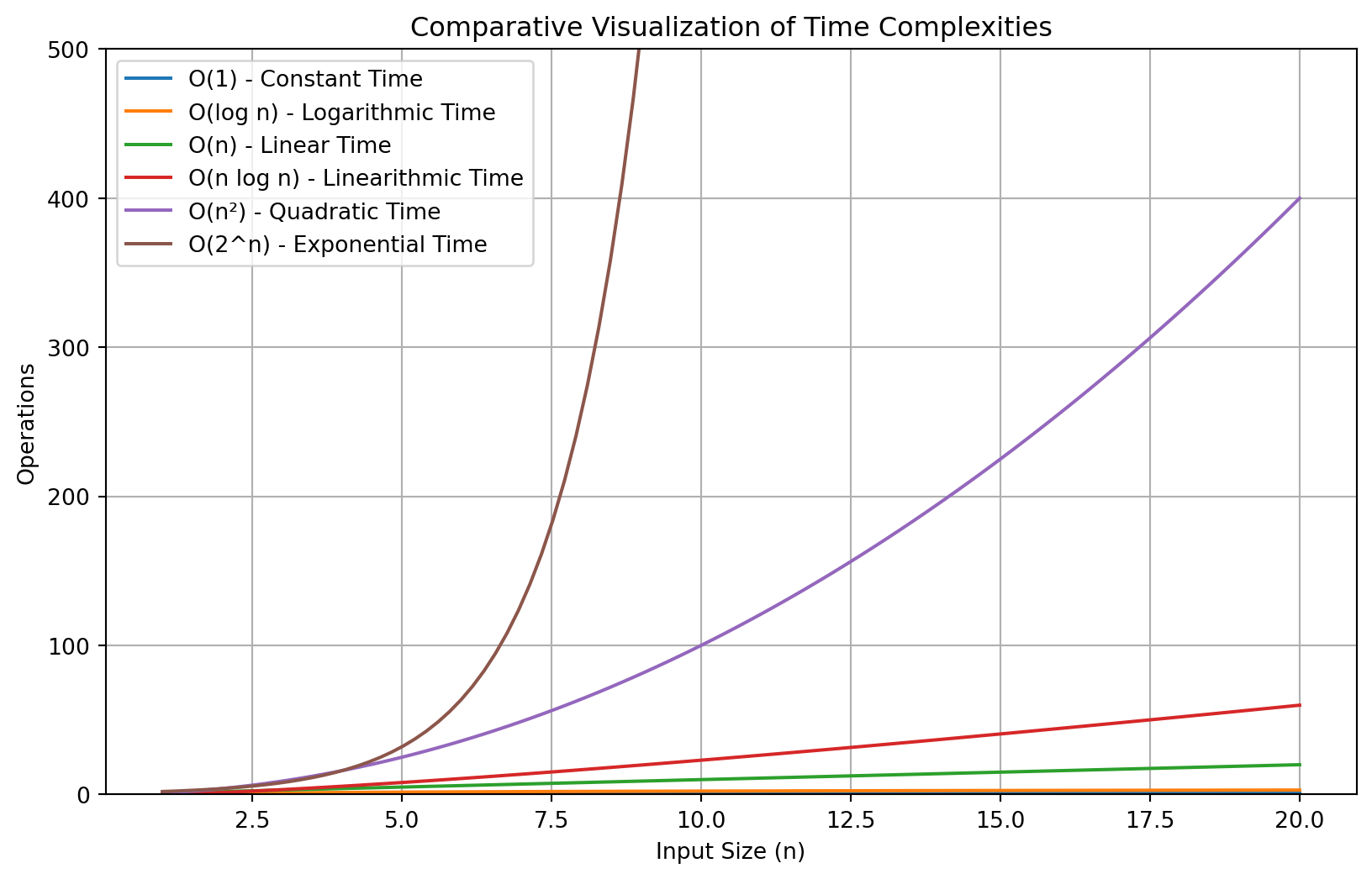
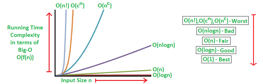
Time Complexities Comparison Table

Complexity	Class Name	Description	Real-World Example	Graph
\(O(1)\)	Constant Time	Always takes the same time regardless of input size	Accessing an element in an array	Flat Line
\(O(\log n)\)	Logarithmic Time	Runtime grows slowly with input size	Binary search in a phone book	Slowly Increasing Curve
\(O(n)\)	Linear Time	Runtime grows directly proportional to input size	Reading through a list of names in a document	Straight Line
\(O(n \log n)\)	Linearithmic Time	Efficient sorting, slower than linear	Efficient sorting algorithms like Merge Sort	Rising Curve
\(O(n^2)\)	Quadratic Time	Runtime grows exponentially with input size	Bubble Sort on a long list of elements	Steep Curve
\(O(2^n)\)	Exponential Time	Runtime doubles with each additional element	Recursive solutions to combinatorial problems	Exponential Curve
\(O(n!)\)	Factorial Time	Runtime grows factorially with input size	Generating all permutations of a list	Extremely Steep Curve

Visualization of Time Complexities

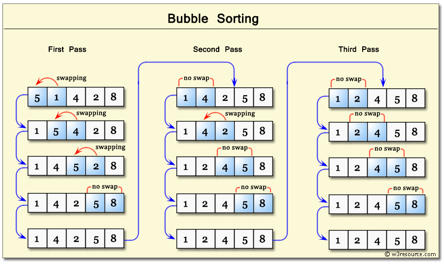
Bubble Sort

Bubbles

Introduction to Bubble Sort

• Bubble Sort is a simple, comparison-based sorting algorithm. It repeatedly steps through a list, compares adjacent elements, and swaps them if they are in the wrong order.
• The smaller elements “bubble” to the top, while larger elements “sink” to the bottom. This process repeats until the list is sorted.

How Bubble Sort Works

1. Start at the beginning of the list.
2. Compare each pair of adjacent elements.
3. If they are in the wrong order, swap them.
4. Repeat this process until no more swaps are needed.

Bubble Sort Swaps

Bubble Sort Flowchart

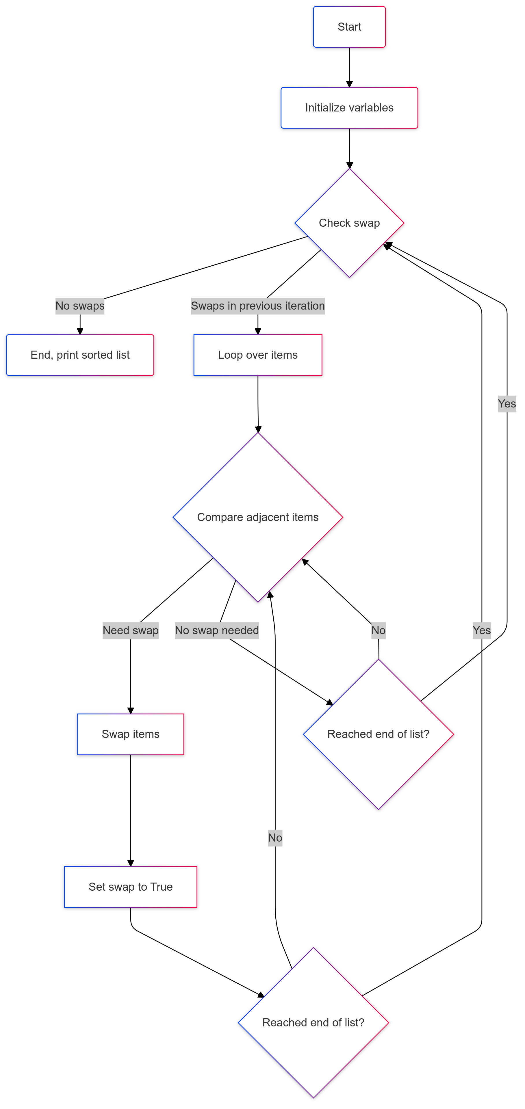
Bubble Sort Flowchart

Bubble Sort Activity

• We need 7-10 student volunteers of different heights to stand in a row.
• Use the Bubble Sort algorithm to sort the volunteers by height from shortest to tallest.
• Compare adjacent volunteers, swap if necessary, and repeat until sorted.

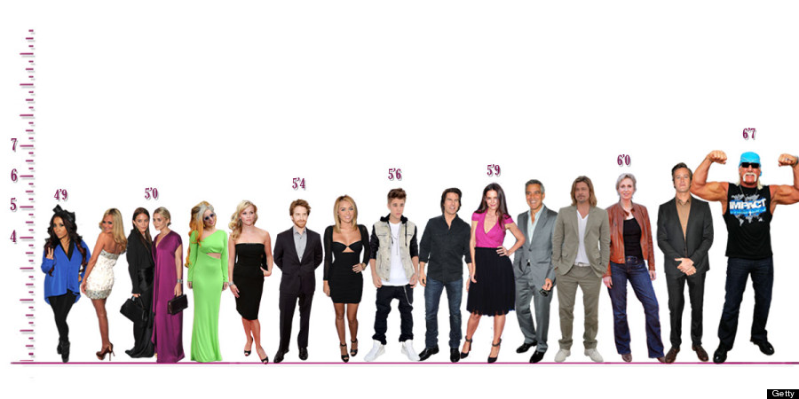
Celebrity Heights

Tracing Bubble Sort Swaps

• Let’s sort the list [5, 1, 4, 2, 8] step-by-step:

1. First Pass:

   • Compare 5 and 1 → Swap → [1, 5, 4, 2, 8]

   • Compare 5 and 4 → Swap → [1, 4, 5, 2, 8]

   • Compare 5 and 4 → Swap → [1, 4, 5, 2, 8]

   • Compare 5 and 2 → Swap → [1, 4, 2, 5, 8]

   • Compare 5 and 8 → No swap.

   • List after first pass: [1, 4, 2, 5, 8]

2. Second Pass:

   • Compare 1 and 4 → No swap.

   • Compare 4 and 2 → Swap → [1, 2, 4, 5, 8]

   • Compare 4 and 5 → No swap.

   • Compare 5 and 8 → No swap.

   • List after second pass: [1, 4, 2, 5, 8]

3. Third Pass:

   • Compare 1 and 2 → No swap.

   • Compare 2 and 4 → Swap → [1, 2, 4, 5, 8]

   • Compare 4 and 5 → No swap.

   • Compare 5 and 8 → No swap.

   • List after third pass: [1, 2, 4, 5, 8]

4. Fourth Pass:

   • Compare 1 and 2 → No swap.

   • Compare 2 and 4 → No swap.

   • Compare 4 and 5 → No swap.

   • Compare 5 and 8 → No swap.

   • List after fourth pass: [1, 2, 4, 5, 8]

The list is now sorted; no further passes needed.

Bubble Sort in Python

Write a Python program to perform a bubble sort

• Input: [5, 1, 4, 2, 8]
• Expected Output: [1, 2, 4, 5, 8]

# Initialize a list of unsorted items
items = [5, 1, 4, 2, 8]

# Determine the number of items in the list
n = len(items)

# Initialize a boolean variable to track swaps
swap = True

# Continue looping while swaps occur
while swap:
    swap = False  # Reset swap flag
    for i in range(1, n):
        if items[i-1] > items[i]:  # Compare adjacent items
            items[i-1], items[i] = items[i], items[i-1]  # Swap if needed
            swap = True  # Set swap flag to True

# Print the sorted list
print(items)

[1, 2, 4, 5, 8]

Time Complexity of Bubble Sort

• Best Case: \(O(n)\) – This occurs when the list is already sorted. In this case, Bubble Sort makes only one pass.

• Worst Case: \(O(n^2)\) – This occurs when the list is in reverse order. Every element needs to be compared and swapped.

Mathematical Derivation of Bubble Sort Complexity (Extra)

Step 1: Algorithm Overview

Bubble sort repeatedly compares adjacent elements and swaps them if they are in the wrong order.

Step 2: Worst-Case Scenario

In the worst-case scenario (when the list is reversed), Bubble Sort must perform comparisons and swaps for nearly every pair of elements.

Step 3: Establishing Complexity

• For each pass, the number of comparisons is \(n-1\), \(n-2\), …, \(1\).
• The total number of comparisons is the sum of the series: \[ (n-1) + (n-2) + \dots + 2 + 1 \]

Step 4: Solving the Sum

The above sum can be simplified using the arithmetic series formula: \[ \frac{n(n-1)}{2} \]

Step 5: Final Complexity

The simplified complexity expression is: \[ \boxed{T(n) = O(n^2)} \]

• This quadratic complexity makes Bubble Sort inefficient for large datasets.
• More efficient sorting algorithms include Merge Sort, Quick Sort, and Heap Sort, with complexities \(O(n \log n)\).

Matrix Multiplication

The Matrix Code

Introduction to Matrix Multiplication

• Matrix Multiplication is an operation that combines two matrices to produce a third matrix.
• Matrices represent data in rows and columns, and multiplying them allows us to transform or process data in powerful ways.

How Matrix Multiplication Works

Example:

Given two matrices \(A\) and \(B\):

\[ A = \begin{bmatrix} 1 & 2 \\ 3 & 4 \end{bmatrix} \quad \text{and} \quad B = \begin{bmatrix} 5 & 6 \\ 7 & 8 \end{bmatrix} \]

Their product \(C = A \times B\) is:

\[ C = \begin{bmatrix} (1 \times 5 + 2 \times 7) & (1 \times 6 + 2 \times 8) \\ (3 \times 5 + 4 \times 7) & (3 \times 6 + 4 \times 8) \end{bmatrix} = \begin{bmatrix} 19 & 22 \\ 43 & 50 \end{bmatrix} \]

Formula:

For each element \(C_{i,j}\) in the resulting matrix: \[ C_{i,j} = \sum_{k=1}^{n} A_{i,k} \times B_{k,j} \]

Where \(A\) is an \(m \times n\) matrix, and \(B\) is an \(n \times p\) matrix.

Notes:

• The product of \(A \times B\) will be of dimension \(𝑚 \times p\).
• The number of columns in matrix \(A\) (i.e., \(n\)) must match the number of rows in matrix \(B\) for the multiplication to be possible.

Matrix Multiplication in Python

Write a Python function matrix_multiply that takes to input matrices, A and B and returns the product of their matrix multiplication

• Example:

A = [[1, 2], [3, 4]]
B = [[5, 6], [7, 8]]
matrix_multiply(A, B)

[[19, 22], [43, 50]]

• Answer:

def matrix_multiply(A, B):
  # Initialize an empty list to store the result of the matrix multiplication
  result = []
  
  # Create a matrix with the same number of rows as A and columns as B, filled with zeros
  for i in range(len(A)):
    row = []  # Initialize a new row
    for j in range(len(B[0])):  # Iterate over columns of B
      row.append(0)  # Append 0 to represent the initial state
    result.append(row)  # Append the row to the result matrix
    
  # Perform matrix multiplication
  for i in range(len(A)):  # Loop over rows of A
    for j in range(len(B[0])):  # Loop over columns of B
      for k in range(len(B)):  # Loop over rows of B (and columns of A)
        # Multiply corresponding elements and add to the current cell in result
        result[i][j] += A[i][k] * B[k][j]
  
  return result  # Return the result matrix

# Example matrices to test the function
A = [[1, 2], [3, 4]]
B = [[5, 6], [7, 8]]
matrix_multiply(A, B)  # Expected output: [[19, 22], [43, 50]]

[[19, 22], [43, 50]]

• Explanation:

1. Matrix Setup: The first loop constructs a result matrix with the appropriate dimensions (rows of \(A\) \(\times\) columns of \(B\)), initialized to zeros.
2. Matrix Multiplication: The nested loops calculate the dot product for each element in the result matrix by summing the products of corresponding elements in each row of \(A\) and column of \(B\).
3. Return Statement: Finally, the function returns the resulting matrix after the multiplication.

Key Points:

• The outer loops traverse the rows and columns.
• The inner loop calculates the dot product between rows of \(A\) and columns of \(B\).

Time Complexity of Matrix Multiplication

• For two matrices, \(A\) of size \(m \times n\) and \(B\) of size \(n \times p\), the time complexity of standard (naive) matrix multiplication is: \(O(m \times n \times p)\)
• If the matrices are square (i.e., \(m = n = p\)), the time complexity simplifies to \(O(n^3)\).

Applications of Matrix Multiplication

• Transformation: In computer graphics, matrix multiplication is used to rotate, scale, or translate objects.
• Data Representation: In machine learning, data is often represented as matrices, such as weights in neural networks.
• Solving Systems of Equations: In linear algebra, matrix multiplication helps solve systems of equations.

Mathematical Derivation of Matrix Multiplication Complexity (Extra)

Step 1: Definition of Matrix Multiplication

Given two matrices \(A\) of size \(m \times n\) and \(B\) of size \(n \times p\), their product \(C = AB\) is an \(m \times p\) matrix, where each element is computed as:

\[ C_{ij} = \sum_{k=1}^{n} A_{ik} B_{kj} \]

Step 2: Counting Operations

To compute a single element \(C_{ij}\), we perform:

• \(n\) multiplications
• \(n - 1\) additions (approximately \(n\))

Thus, roughly \(2n\) operations per element.

Step 3: Total Number of Operations

Since there are \(m \times p\) elements in the resulting matrix, the total number of operations is: \[ 2n \times m \times p \]

Step 4: Simplifying the Complexity

Dropping constant factors, the complexity becomes: \[ \boxed{T(m,n,p) = O(mnp)} \]

Step 5: Final Complexity

The complexity of multiplying two matrices is cubic in general (for square matrices \(m = n = p\)): \[ \boxed{T(n) = O(n^3)} \]

• This cubic complexity makes matrix multiplication computationally intensive for large matrices.
• Advanced algorithms such as Strassen’s algorithm reduce complexity to approximately \(O(n^{2.81})\).

Recursive Fibonacci

Nautilus shell

Recursive Fibonacci Sequence

• Write a recursive function that calculates the Fibonacci number for a given \(n\).
• Test it with small values like \(n = 5\) and \(n = 6\).

def fibonacci(n):
    if n <= 1:
        return n
    else:
        return fibonacci(n - 1) + fibonacci(n - 2)

print(fibonacci(5))  # Output: 5
print(fibonacci(6))  # Output: 8

5
8

Recursive Tree Visualization

• Draw the recursion tree to visualize the recursive calls \(n = 5\):

fibonacci(5)
   |
   +-- fibonacci(4)
   |      |
   |      +-- fibonacci(3)
   |      |      |
   |      |      +-- fibonacci(2)
   |      |      |      +-- fibonacci(1)
   |      |      |      +-- fibonacci(0)
   |      |      +-- fibonacci(1)
   |      +-- fibonacci(2)
   |             +-- fibonacci(1)
   |             +-- fibonacci(0)
   +-- fibonacci(3)
          |
          +-- fibonacci(2)
          |      +-- fibonacci(1)
          |      +-- fibonacci(0)
          +-- fibonacci(1)

• Notice how the same values are recomputed multiple times.

Counting the Number of Recursive Calls

• Modify the fibonacci function to count the number of recursive calls.

def fibonacci(n):
    global call_count
    call_count += 1
    if n <= 1:
        return n
    else:
        return fibonacci(n - 1) + fibonacci(n - 2)

• Number of calls for fibonacci(5)

n = 5
call_count = 0
fibonacci(n)
print("Number of recursive calls for n = ", 5, ": " , call_count)

Number of recursive calls for n =  5 :  15

• Number of calls for fibonacci(6)

n = 6
call_count = 0
fibonacci(n)
print("Number of recursive calls for n = ", 6, ": " , call_count)

Number of recursive calls for n =  6 :  25

Visualizing the Number of Recursive Calls

• Count the recursive calls for multiple values of \(n\) and plot the results.

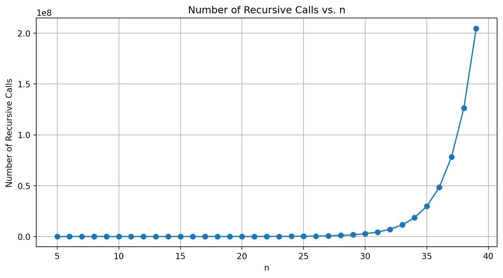
Time Complexity of Fibonacci

• Every call to fibonacci(n) splits into two subproblems: fibonacci(n-1) and fibonacci(n-2).
• The total number of nodes in the tree is approximately \(2^n\), leading to the time complexity of \(O(2^n)\).
• Implication: Highly inefficient for large \(n\) due to overlapping subproblems and repeated calculations.

Mathematical Derivation of Recursive Fibonacci Complexity (Extra)

Step 1: Recursive Definition

The Fibonacci function is defined as: \[ F(n) = F(n-1) + F(n-2), \quad F(0)=0, \quad F(1)=1 \]

Step 2: Counting Recursive Calls

Each call to fibonacci(n) creates two additional calls:

• fibonacci(n-1) and fibonacci(n-2)
• This forms a binary tree of recursive calls.

Step 3: Establishing the Recurrence Relation

The time complexity \(T(n)\) satisfies:

\[ T(n) = T(n-1) + T(n-2) + O(1) \]

Step 4: Solving the Recurrence

This recurrence relation closely resembles the Fibonacci series itself. The number of recursive calls made by the algorithm aligns with the Fibonacci numbers. Specifically, the number of calls grows as: \[ T(n) \approx F(n+1) \]

Since the Fibonacci numbers grow exponentially, this can be approximated by: \[ F(n) \approx \frac{\phi^n}{\sqrt{5}}, \quad \text{where } \phi = \frac{1 + \sqrt{5}}{2} \approx 1.618034 \text{ (The Golden Ratio)} \]

Thus, the complexity is: \[ T(n) \approx O(\phi^n) \]

Step 5: Final Complexity

The recursive Fibonacci algorithm has an exponential time complexity: \[ \boxed{T(n) = O(2^n)} \]

• The exponential nature of this complexity makes the naive recursive Fibonacci implementation impractical for large values of \(n\).
• More efficient approaches, like iterative solutions or memoization, significantly improve performance.

Summary

[Source: Big O Notation Tutorial – A Guide to Big O Analysis]