flowchart LR
    A[Problem] --> B{Analytical<br/>Solution<br/>Feasible?}
    B -->|Yes| C[Derive Exact<br/>Probability]
    B -->|No| D[Monte Carlo<br/>Simulation]
    C --> E[Validate with<br/>Simulation]
    D --> F[Generate Random<br/>Samples]
    F --> G[Count<br/>Successes]
    G --> H[Calculate<br/>Proportion]
    H --> I[Quantify<br/>Uncertainty]
    I --> J[Report Results<br/>with CI]
    E --> J

    style A fill:#FFE082,color:#000000
    style C fill:#81C784,color:#000000
    style D fill:#64B5F6,color:#000000
    style J fill:#BA68C8,color:#FFFFFF
    style E fill:#4DB6AC,color:#000000
Probability Simulation in Python
Monte Carlo Methods, Random Number Generation, and Statistical Convergence
2025-11-05
Learning Objectives
By the end of this lecture, you will be able to:
Core Concepts:
- Understand Monte Carlo simulation principles and theoretical foundations
- Master the Law of Large Numbers and its role in simulation
- Apply standard error formulas to quantify estimation uncertainty
- Implement probability simulations using Python’s random module
Advanced Techniques:
- Perform convergence analysis to assess simulation accuracy
- Calculate and interpret empirical vs. theoretical standard deviation
- Visualize simulation results and convergence patterns
- Apply the complement rule and sampling methods in simulations
Success Criteria: You will build reliable simulations based on statistical principles that accurately approximate theoretical probabilities, properly quantify estimation uncertainty, and demonstrate convergence to theoretical values.
Introduction to Probability Simulation
Probability simulation uses computational methods to approximate solutions to probabilistic problems by generating random outcomes and analyzing their frequency.
This approach offers a practical computational tool in statistics when analytical solutions are unavailable or computationally prohibitive.
What are Monte Carlo Methods?
Monte Carlo methods are a broad class of computational algorithms that rely on repeated random sampling to obtain numerical results. The key idea is to use randomness to solve problems that might be deterministic in principle.
Core principle: When a problem is too complex to solve analytically, we can:
- Generate many random samples following the problem’s probability distribution
- Compute the desired quantity for each sample
- Aggregate the results to approximate the true answer
The name “Monte Carlo” reflects the element of chance in casino games. Here, however, randomness serves as a problem-solving tool rather than a source of uncertainty.
Simple analogy: Imagine trying to estimate the area of an irregularly shaped lake. Instead of complex geometric calculations, you could randomly throw darts at a map and count what proportion land in the lake. With enough darts, this random process gives an accurate estimate.
Historical Context
The modern Monte Carlo method was formalized in the 1940s by mathematicians Stanislaw Ulam, John von Neumann, and Nicholas Metropolis during the Manhattan Project. The name “Monte Carlo” was coined by Metropolis, referencing the famous casino in Monaco.
However, the conceptual foundations extend back to Georges-Louis Leclerc, Comte de Buffon, who in 1777 posed Buffon’s needle problem, one of the earliest problems in geometric probability that can be solved through simulation.
Why Simulation Matters
Simulation methods enable probabilistic analysis when analytical solutions are infeasible:
- Verify theoretical calculations through empirical approximation
- Solve complex problems where closed-form solutions do not exist
- Model real-world randomness in systems with multiple stochastic components
- Estimate rare event probabilities through importance sampling
- Understand convergence behavior and sampling variability
Without simulation, many practical problems in fields ranging from risk assessment to quantum mechanics would be difficult or impossible to solve analytically. Random sampling approximates probabilities in complex scenarios where exact calculations are infeasible.
Monte Carlo Decision Framework
This framework illustrates the decision process: always attempt analytical solutions first, then use simulation either for validation or when analytical methods fail. The simulation path follows a systematic workflow ending with uncertainty quantification.
The Anatomy of a Simulation Study
graph TB
    S["Simulation Study"] --> T["Theoretical Foundation"]
    S --> M["Model Construction"]
    S --> I["Implementation"]
    S --> V["Validation"]
    S --> A["Analysis"]

    T --> TL["Law of Large Numbers"]
    T --> TS["Standard Error Theory"]

    M --> MD["Specify random mechanisms"]
    M --> MP["Define success criteria"]

    I --> IR["Generate random trials"]
    I --> IC["Count successes"]

    V --> VC["Compare with theory"]
    V --> VT["Convergence analysis"]

    A --> AI["Interpret results"]
    A --> AU["Quantify uncertainty"]

    style S fill:#2E7D32,color:#FFFFFF
    style T fill:#1565C0,color:#FFFFFF
    style M fill:#1565C0,color:#FFFFFF
    style I fill:#E65100,color:#FFFFFF
    style V fill:#E65100,color:#FFFFFF
    style A fill:#6A1B9A,color:#FFFFFF
Theoretical Foundations
The Law of Large Numbers
The Law of Large Numbers provides the mathematical foundation ensuring that simulation methods converge to accurate results as sample size increases.
Intuitive Explanation
The Law of Large Numbers states that if you repeat a random experiment many times, the average of your results will approach the expected (true) value. The more trials you run, the closer you get to the true value.
Example: If you flip a fair coin, you expect 50% heads. With 10 flips, you might get 60% or 40% heads. With 100 flips, you might get 52% or 48%. With 10,000 flips, you will be very close to 50%. With a million flips, you will be extremely close to 50%.
Formal Statement
Let \(X_1, X_2, \ldots, X_n\) be random variables satisfying:
Assumptions:
- Independence: \(X_i \perp X_j\) for all \(i \neq j\) (outcomes do not influence each other)
- Identical Distribution: \(X_i \sim F\) for all \(i\) (same probability rules apply)
- Finite Expectation: \(E[|X_i|] = \mu < \infty\) (expected value exists and is finite)
Under these conditions, the sample mean converges to the true mean.
The sample mean is:
\[ \bar{X}_n = \frac{1}{n}\sum_{i=1}^{n}X_i \]
Reading this: \(\bar{X}_n\) (read as “X-bar sub n”) is the average of all \(n\) trials. The notation \(\sum_{i=1}^{n}X_i\) means “sum up all the \(X\) values from trial 1 to trial \(n\).”
As \(n\) increases, \(\bar{X}_n\) converges in probability to \(\mu\):
\[ \lim_{n \to \infty} P(|\bar{X}_n - \mu| > \varepsilon) = 0 \quad \text{for any } \varepsilon > 0 \]
Reading this: As \(n\) approaches infinity (gets very large), the probability that our average \(\bar{X}_n\) differs from the true mean \(\mu\) by more than any small amount \(\varepsilon\) (epsilon) approaches zero. In other words, the chance of being wrong becomes vanishingly small.
This is the Weak Law of Large Numbers. The Strong Law provides an even stronger guarantee:
\[ P\left(\lim_{n \to \infty} \bar{X}_n = \mu\right) = 1 \]
Reading this: With probability 1 (certainty), the average will eventually equal the true mean as \(n\) grows.
Application to Probability Simulation
In probability simulation, we apply the Law of Large Numbers to estimate probabilities.
Bernoulli Trials Framework
Each simulation trial generates a Bernoulli random variable:
\[ X_i = \begin{cases} 1 & \text{if trial } i \text{ is successful} \\ 0 & \text{otherwise} \end{cases} \]
The expected value is \(E[X_i] = p\), where \(p\) is the true probability of success.
Sample Proportion as Estimator
The sample proportion after \(n\) trials is:
\[ \hat{p}_n = \frac{1}{n}\sum_{i=1}^{n}X_i = \frac{\text{number of successes}}{n} \]
By the Law of Large Numbers, \(\hat{p}_n \xrightarrow{P} p\) as \(n \to \infty\).
Conclusion: Our simulation estimate \(\hat{p}_n\) is guaranteed to converge to the true probability \(p\) as we increase the number of trials. This theorem justifies the Monte Carlo approach.
From Theory to Practice: Connecting the Pieces
We have established three theoretical foundations:
- Law of Large Numbers: Guarantees \(\hat{p}_n \to p\) as \(n \to \infty\)
- Standard Error Formula: Quantifies uncertainty as \(\text{SE} = \sqrt{p(1-p)/n}\)
- Convergence Rate: Precision improves at rate \(O(n^{-1/2})\)
These theoretical guarantees translate into practical simulation guidelines:
| Theoretical Principle | Practical Implication |
|---|---|
| LLN convergence | More trials yield more accurate estimates |
| SE formula | Can predict precision before running simulation |
| \(O(n^{-1/2})\) rate | Quadruple trials to halve error |
| Maximum variance at \(p=0.5\) | Coin flip requires most trials for given precision |
| CLT normality | Can construct valid confidence intervals |
The remainder of this lecture demonstrates these principles through implementation.
Standard Error and Convergence Rate
While the Law of Large Numbers guarantees convergence, the standard error quantifies how much uncertainty remains for a given sample size.
Standard Error Formula
For a Bernoulli random variable with success probability \(p\), the standard error of the sample proportion is:
\[ \text{SE}(\hat{p}_n) = \sqrt{\frac{p(1-p)}{n}} \]
This formula reveals fundamental relationships about convergence:
Key Properties
- Inverse square root relationship: \(\text{SE}(\hat{p}_n) = O(n^{-1/2})\)
- To halve the standard error, we need four times as many trials
- To gain one decimal place of precision, we need 100 times as many trials
- Maximum variance at \(p = 0.5\): Standard error is largest when \(p = 0.5\)
- Events with extreme probabilities require fewer trials for given precision
- For \(p = 0.5\) and \(n = 10,000\): \(\text{SE} \approx 0.005\) (about \(\pm 0.01\) for 95% confidence)
- Confidence intervals: By the Central Limit Theorem, for sufficiently large \(n\) (typically \(n \geq 30\)), \(\hat{p}_n\) is approximately normally distributed with mean \(p\) and variance \(p(1-p)/n\). Therefore: \[ \hat{p}_n \pm 1.96 \cdot \text{SE}(\hat{p}_n) \] provides an approximate 95% confidence interval for \(p\)
Understanding Standard Error
The standard error formula \(\text{SE} = \sqrt{p(1-p)/n}\) tells us three important things:
Precision of estimates: Smaller SE means more precise estimates. Since \(\text{SE} \propto 1/\sqrt{n}\), we must quadruple the number of trials to halve the standard error.
Required sample size: We can determine the needed sample size for desired precision. For example, to achieve \(\text{SE} = 0.01\), we need approximately \(n = 2,500\) trials (when \(p = 0.5\)).
Confidence intervals: The SE allows us to construct confidence intervals as \(\hat{p} \pm 1.96 \cdot \text{SE}\) for 95% confidence, quantifying the uncertainty in our estimates.
Two Types of Standard Deviation
In convergence analysis, we distinguish between theoretical predictions and empirical observations:
Theoretical Standard Error (Expected)
What probability theory predicts the standard deviation should be (using the true probability \(p\)):
\[ \sigma_n = \sqrt{\frac{p(1-p)}{n}} \]
Where:
- \(p\) is the true probability (parameter, not estimated)
- \(n\) is the number of trials per simulation
- Derived from binomial distribution theory: \(\text{Var}(\hat{p}_n) = p(1-p)/n\)
Purpose: Provides the theoretical benchmark for expected variability. Note that this requires knowing the true \(p\), which in practice we estimate using \(\hat{p}_n\).
Empirical Standard Deviation (Observed)
What we actually measure from running multiple simulations:
\[ s_n = \sqrt{\frac{1}{R-1}\sum_{r=1}^{R}(\hat{p}_{n,r} - \bar{p}_n)^2} \]
Where:
- \(\hat{p}_{n,r}\) is the probability estimate from replication \(r\)
- \(\bar{p}_n\) is the mean across \(R\) replications (typically \(R = 100\))
- Calculated from actual simulation data
Purpose: Validates that our simulation behaves as theory predicts.
Validation Through Comparison
For a correctly implemented simulation, the empirical standard deviation \(s_n\) should closely match the theoretical standard error \(\sigma_n\):
\[ s_n \approx \sigma_n \]
Diagnostic Framework
| Observation | Interpretation | Action |
|---|---|---|
| \(s_n \approx \sigma_n\) | Simulation valid | Proceed with confidence |
| \(s_n \gg \sigma_n\) | Excessive variance; implementation error | Debug code logic |
| \(s_n \ll \sigma_n\) | Insufficient variance; too few replications | Increase \(R\) |
| Pattern mismatch | Model misspecification | Revisit assumptions |
Key Principle: Never simply trust that simulation code works. Always verify that it produces the variability predicted by theory. The agreement between empirical and theoretical standard deviations serves as a critical validation check, ensuring that theoretical predictions match empirical observations.
Conceptual Checkpoint: Theoretical Foundations
Before proceeding to implementation, verify your understanding:
- What does the Law of Large Numbers guarantee for our simulations?
Answer: The LLN guarantees that \(\hat{p}_n\) converges to the true \(p\) as \(n \to \infty\)
- How does standard error change when we quadruple the sample size?
Answer: Quadrupling \(n\) halves the SE (since \(\text{SE} \propto 1/\sqrt{n}\))
- Why is the ratio of empirical SD to theoretical SE important for validation?
Answer: The ratio \(s_n / \sigma_n \approx 1\) confirms the simulation is correctly implemented
- For \(p=0.5\) and \(n=10,000\), what precision should we expect?
Answer: \(\text{SE} = \sqrt{0.5 \times 0.5 / 10,000} = 0.005\), giving 95% CI width of approximately \(\pm 0.01\)
Random Number Generation
Python’s random Module
The random module provides pseudorandom number generation capabilities based on the Mersenne Twister algorithm, which has a period of \(2^{19937} - 1\) and passes numerous statistical tests for randomness.
Core Functionality
Python’s random number generation serves three primary purposes in simulation:
- Generate uniform random values for basic probabilistic events
- Sample from probability distributions to model complex phenomena
- Perform random operations on data structures for shuffling and selection
The module implements a deterministic algorithm that produces sequences appearing random for practical purposes. For cryptographic applications requiring true randomness, the secrets module should be used instead.
Random Module Function Hierarchy
graph TB
    RNG[Random Number<br/>Generation]

    RNG --> U[Uniform<br/>Distribution]
    RNG --> D[Discrete<br/>Events]
    RNG --> S[Sampling<br/>Operations]
    RNG --> C[Continuous<br/>Distributions]

    U --> U1["random()"]
    U --> U2["uniform(a,b)"]

    D --> D1["randint(a,b)"]
    D --> D2["randrange(...)"]

    S --> S1["choice(seq)"]
    S --> S2["sample(pop,k)"]
    S --> S3["choices(...,weights)"]
    S --> S4["shuffle(seq)"]

    C --> C1["gauss(μ,σ)"]
    C --> C2["expovariate(λ)"]

    style RNG fill:#1565C0,color:#FFFFFF
    style U fill:#7CB342,color:#FFFFFF
    style D fill:#7CB342,color:#FFFFFF
    style S fill:#FB8C00,color:#FFFFFF
    style C fill:#AB47BC,color:#FFFFFF
This taxonomy organizes the random module’s functions by their primary purpose, facilitating selection of appropriate methods for different simulation scenarios.
Important Distinction: Pseudorandom numbers are deterministic sequences that appear random. True random numbers require physical entropy sources. For statistical simulation, pseudorandom generation is both sufficient and preferable due to reproducibility.
Essential Methods of the random Module
The following table organizes key methods by their primary use in probability simulation:
Basic Random Number Generation
| Method | Description | Use Case | Example |
|---|---|---|---|
random() |
Returns float in \([0.0, 1.0)\) | Foundation for all random events; convert to probabilities | random.random() < 0.3 (30% probability) |
uniform(a, b) |
Returns float uniformly distributed in \([a, b]\) | Continuous random variables with equal likelihood | random.uniform(5.0, 10.0) (temperature) |
seed(a) |
Sets random seed for reproducibility | Scientific computing, debugging, testing | random.seed(42) before simulations |
Why these matter: random() is the fundamental building block. All probability events can be modeled by checking if random() falls in certain ranges. The seed() function makes simulations reproducible.
Integer Random Selection
| Method | Description | Use Case | Example |
|---|---|---|---|
randint(a, b) |
Returns random integer in \([a, b]\) inclusive | Discrete uniform events (dice, cards) | random.randint(1, 6) (die roll) |
randrange(start, stop, step) |
Random integer from range with optional step | Sampling with gaps or patterns | random.randrange(0, 100, 5) (multiples of 5) |
Why these matter: Use when outcomes are discrete integers. randint is simpler for basic cases; randrange provides more control.
Sampling from Collections
| Method | Description | Use Case | Example |
|---|---|---|---|
choice(seq) |
Returns single random element from sequence | Selecting one item from a list | random.choice(['red', 'blue', 'green']) |
sample(pop, k) |
Returns \(k\) unique random elements (no replacement) | Drawing without replacement (lottery, card dealing) | random.sample(range(1, 50), 6) (lottery) |
choices(pop, weights, k) |
Returns \(k\) random elements with replacement and optional weights | Repeated sampling, weighted probabilities | random.choices(['A', 'B'], weights=[0.7, 0.3], k=100) |
shuffle(seq) |
Shuffles list in-place | Randomizing order (card deck, experimental conditions) | random.shuffle(deck) |
Why these matter: These handle common simulation scenarios. Use choice for one item, sample when selections must be unique, choices when repetition is allowed or probabilities differ, and shuffle to randomize order.
Statistical Distributions
| Method | Description | Use Case | Example |
|---|---|---|---|
gauss(mu, sigma) |
Returns random value from normal (Gaussian) distribution | Modeling measurements, errors, natural phenomena | random.gauss(100, 15) (IQ scores) |
Why this matters: Many real-world quantities follow normal distributions. Use when simulating measurements, biological traits, or errors.
Time Complexity Note: All methods except shuffle run in \(O(1)\) constant time. shuffle runs in \(O(n)\) time where \(n\) is the list length. Sampling methods run in \(O(k)\) time where \(k\) is the number of items requested.
Reproducibility Through Seeding
Setting a random seed ensures reproducible results, which is critical for debugging, testing, and scientific reproducibility.
What this demonstration shows: When we set the same random seed (random.seed(42)), we get identical sequences of “random” numbers. This proves that pseudorandom generators are deterministic—they produce the same output given the same starting state. Without setting a seed, each run produces different numbers, which is useful for production but problematic for debugging and scientific validation.
import random

def demonstrate_seeding():
    """
    Demonstrates the importance of random seed for reproducibility.

    Returns:
        dict: Results showing reproducible vs non-reproducible sequences
    """
    results = {}

    # Reproducible sequence
    random.seed(42)
    results['first_sequence'] = [random.random() for _ in range(5)]

    # Reset seed - produces identical sequence
    random.seed(42)
    results['repeated_sequence'] = [random.random() for _ in range(5)]

    # No seed - produces different sequence
    results['different_sequence'] = [random.random() for _ in range(5)]

    return results

# Execute demonstration
demo_results = demonstrate_seeding()
print("First sequence:     ", [f"{x:.6f}" for x in demo_results['first_sequence']])
print("Repeated sequence:  ", [f"{x:.6f}" for x in demo_results['repeated_sequence']])
print("Different sequence: ", [f"{x:.6f}" for x in demo_results['different_sequence']])
print(f"\nFirst == Repeated: {demo_results['first_sequence'] == demo_results['repeated_sequence']}")
print(f"First == Different: {demo_results['first_sequence'] == demo_results['different_sequence']}")
First sequence: ['0.639427', '0.025011', '0.275029', '0.223211', '0.736471']
Repeated sequence: ['0.639427', '0.025011', '0.275029', '0.223211', '0.736471']
Different sequence: ['0.676699', '0.892180', '0.086939', '0.421922', '0.029797']
First == Repeated: True
First == Different: FalseExecution Analysis: The first two sequences are identical because both use seed(42), resetting the pseudorandom number generator to the same initial state. The third sequence differs because it continues from the current generator state without reseeding. This demonstrates that pseudorandom sequences are deterministic and reproducible when seeded consistently.
Best Practice: Always set a seed when debugging simulations or preparing results for publication to ensure reproducibility. However, for final production runs, test multiple seeds to ensure results are not seed-dependent.
Simulation Methodology
General Simulation Framework
Having established the theoretical foundations, we now define the systematic process for implementing probability simulations.
Core Algorithm Structure
All probability simulations follow this pattern:
- Initialize: Set random seed for reproducibility
- Generate: Create \(n\) independent random trials
- Evaluate: Apply success criterion to each trial
- Count: Accumulate successful outcomes
- Estimate: Calculate \(\hat{p}_n = \frac{\text{successes}}{n}\)
- Quantify: Compute \(\text{SE}(\hat{p}_n) = \sqrt{\frac{\hat{p}_n(1-\hat{p}_n)}{n}}\)
This framework embodies the theoretical principles we have established: the Law of Large Numbers guarantees convergence, and the standard error quantifies remaining uncertainty.
Implementation Template
We now translate the theoretical framework into a reusable Python function template. This template serves as the foundation for all simulation exercises that follow, embodying the six-step algorithm we outlined: initialize, generate, evaluate, count, estimate, and quantify uncertainty.
The function below demonstrates professional programming practices including comprehensive documentation, proper parameter handling, and structured output. While this example simulates a simple 50% probability event (like a fair coin), you will adapt this template for more complex scenarios by modifying the success criterion.
What to observe in this code:
- Input design: Accepts both sample size and optional random seed for reproducibility
- Process flow: Follows our established six-step framework explicitly
- Output structure: Returns a dictionary containing all relevant results (estimate, counts, uncertainty measures)
- Validation: Compares simulation results with theoretical predictions
import random

def simulate_probability(n_trials, random_seed=None):
    """
    Template for probability simulation functions.

    This implementation follows the theoretical framework:
    - Law of Large Numbers ensures convergence
    - Standard error quantifies uncertainty
    - Seeding ensures reproducibility

    Args:
        n_trials (int): Number of simulation trials to run
        random_seed (int, optional): Seed for reproducibility

    Returns:
        dict: Contains probability estimate, count, and standard error
    """
    # Step 1: Initialize with seed
    if random_seed is not None:
        random.seed(random_seed)

    # Step 2-4: Generate, evaluate, and count
    successes = 0
    for trial in range(n_trials):
        # Generate random event
        outcome = random.random()

        # Evaluate success criterion (placeholder)
        if outcome < 0.5:
            successes += 1

    # Step 5: Calculate probability estimate
    probability_estimate = successes / n_trials

    # Step 6: Quantify uncertainty
    standard_error = (probability_estimate * (1 - probability_estimate) / n_trials) ** 0.5

    return {
        'probability': probability_estimate,
        'successes': successes,
        'trials': n_trials,
        'std_error': standard_error,
        'ci_lower': probability_estimate - 1.96 * standard_error,
        'ci_upper': probability_estimate + 1.96 * standard_error
    }

# Demonstration
n = 100000
result = simulate_probability(n, random_seed=42)
print(f"Simulation with {n:,} trials:")
print(f"  Estimated probability: {result['probability']:.6f}")
print(f"  Standard error: {result['std_error']:.6f}")
print(f"  95% Confidence interval: [{result['ci_lower']:.6f}, {result['ci_upper']:.6f}]")
print(f"\nTheoretical probability: 0.500000")
print(f"Theoretical standard error: {(0.5 * 0.5 / n)**0.5:.6f}")
Simulation with 100,000 trials:
Estimated probability: 0.499340
Standard error: 0.001581
95% Confidence interval: [0.496241, 0.502439]
Theoretical probability: 0.500000
Theoretical standard error: 0.001581Execution Analysis: This template demonstrates the complete simulation framework. The function returns not just a point estimate but also quantifies uncertainty through standard error and confidence intervals. The comparison with theoretical values validates the implementation.
Applied Probability Simulations
Problem-Solving Methodology
For each probability problem, we apply the following systematic approach:
- Analytical solution: Derive the exact probability using mathematical theory
- Simulation design: Translate the problem into random trial generation
- Implementation: Write code following our established framework
- Validation: Compare simulation results with analytical solution
This methodology ensures that simulation serves as both a computational tool and a means of validating theoretical understanding.
Exercise Progression
The exercises in this lecture build progressively in complexity:
- Exercise 1 (Coin toss): Single Bernoulli trial with comprehensive convergence analysis
- Exercise 2 (Dice rolling): Compound events and the complement rule
- Exercise 3 (Drawing balls): Sampling without replacement
Each exercise introduces new probabilistic concepts while reinforcing the simulation framework. The convergence analysis in Exercise 1 provides a complete demonstration of the theoretical principles underlying all simulation methods.
Exercise 1: Single Coin Toss
Problem: Calculate the probability of obtaining a head when tossing a fair coin once.
Analytical Solution
For a fair coin, each outcome has equal probability. The sample space is \(S = \{\text{H}, \text{T}\}\) with \(|S| = 2\).
The probability of obtaining a head is given by the ratio of favorable outcomes to total outcomes:
\[ P(\text{Head}) = \frac{|\{\text{H}\}|}{|S|} = \frac{1}{2} = 0.5 \]
Theoretical standard error for \(n\) trials:
\[ \text{SE} = \sqrt{\frac{0.5 \times 0.5}{n}} = \frac{0.5}{\sqrt{n}} \]
For \(n = 100,000\): \(\text{SE} \approx 0.0016\), giving 95% CI of approximately \(0.5 \pm 0.003\).
Conclusion: The theoretical probability is exactly \(P(\text{Head}) = 0.5\) or \(50\%\).
Exercise 1: Simulation Implementation
Implementation Strategy
What we will simulate: We will generate 100,000 independent coin tosses and count how many result in heads.
How we will implement it:
- Generate random outcomes: Use
random.choice(['H', 'T'])to randomly select either ‘H’ (heads) or ‘T’ (tails) for each toss - Count successes: Count how many tosses result in ‘H’
- Calculate estimate: Divide number of heads by total trials to get \(\hat{p}\)
- Quantify uncertainty: Compute standard error as \(\text{SE} = \sqrt{\hat{p}(1-\hat{p})/n}\)
- Construct confidence interval: Report \(\hat{p} \pm 1.96 \cdot \text{SE}\) for 95% confidence
Key implementation detail: We use random.seed(42) to ensure reproducible results. The choice() function randomly selects one element from the list with equal probability.
import random

def simulate_coin_toss(n_trials, random_seed=42):
    """
    Simulates fair coin tosses to estimate probability of heads.

    Theoretical Foundation:
        - Each trial is Bernoulli(p=0.5) random variable
        - Sample proportion converges to true p by Law of Large Numbers
        - Standard error: SE = sqrt(p(1-p)/n) = sqrt(0.25/n)
        - 95% CI: p̂ ± 1.96·SE (by Central Limit Theorem for large n)

    Implementation:
        - Uses random.choice(['H', 'T']) for each trial
        - Counts tosses that result in 'H' (heads)
        - Calculates proportion and quantifies uncertainty

    Parameters
    ----------
    n_trials : int
        Number of independent coin tosses to simulate
    random_seed : int, default=42
        Seed for reproducible random number generation

    Returns
    -------
    dict
        Results dictionary with keys:
        - 'probability': Estimated P(heads)
        - 'successes': Count of heads observed
        - 'trials': Number of trials performed
        - 'std_error': Standard error of estimate
        - 'ci_lower': Lower bound of 95% CI
        - 'ci_upper': Upper bound of 95% CI

    Examples
    --------
    >>> result = simulate_coin_toss(10000, random_seed=42)
    >>> print(f"P(heads) ≈ {result['probability']:.4f}")
    P(heads) ≈ 0.5012

    Notes
    -----
    For fair coin (p=0.5), theoretical SE ≈ 0.5/√n.
    With n=100,000, expect SE ≈ 0.0016.
    Empirical SD across replications should match theoretical SE.
    """
    random.seed(random_seed)

    # Count heads using choice
    heads = sum(1 for _ in range(n_trials) if random.choice(['H', 'T']) == 'H')

    # Calculate probability estimate
    prob_heads = heads / n_trials

    # Quantify uncertainty
    std_error = (prob_heads * (1 - prob_heads) / n_trials) ** 0.5

    return {
        'probability': prob_heads,
        'successes': heads,
        'trials': n_trials,
        'std_error': std_error,
        'ci_lower': prob_heads - 1.96 * std_error,
        'ci_upper': prob_heads + 1.96 * std_error
    }

# Run simulation
n_trials = 100000
result = simulate_coin_toss(n_trials)
theoretical_prob = 0.5
theoretical_se = (0.5 * 0.5 / n_trials) ** 0.5

print(f"Simulation Results ({n_trials:,} trials):")
print(f"  Heads obtained: {result['successes']:,}")
print(f"  Estimated P(Head): {result['probability']:.6f}")
print(f"  Standard error: {result['std_error']:.6f}")
print(f"  95% CI: [{result['ci_lower']:.6f}, {result['ci_upper']:.6f}]")
print(f"\nTheoretical Values:")
print(f"  P(Head): {theoretical_prob:.6f}")
print(f"  Standard error: {theoretical_se:.6f}")
print(f"  Absolute error: {abs(result['probability'] - theoretical_prob):.6f}")
Simulation Results (100,000 trials):
Heads obtained: 50,062
Estimated P(Head): 0.500620
Standard error: 0.001581
95% CI: [0.497521, 0.503719]
Theoretical Values:
P(Head): 0.500000
Standard error: 0.001581
Absolute error: 0.000620Execution Analysis: The simulation generates \(100,000\) independent coin tosses using random.choice(['H', 'T']), which randomly selects either ‘H’ or ‘T’ with equal probability. We count tosses that result in ‘H’. The estimated probability should be close to \(0.5\), typically within \(\pm 0.003\) (two standard errors). The observed standard error closely matches the theoretical value, validating our implementation. The 95% confidence interval should contain the true probability \(0.5\) with high probability.
Exercise 1: Convergence Analysis
Now we perform a comprehensive convergence analysis to verify that the coin flip simulation behaves according to theoretical predictions.
What this analysis does: We test 30 different sample sizes (from 10 to 100,000 trials) and run 100 independent simulations at each size. This allows us to observe how the mean estimate converges to the true probability (0.5) and verify that the empirical standard deviation matches the theoretical standard error predictions. The analysis provides empirical evidence that our simulation correctly implements the theoretical framework.
import numpy as np

def coin_toss_convergence(max_trials):
    """
    Comprehensive convergence analysis for coin toss simulation.

    This analysis:
    - Tests 30 sample sizes from 10 to max_trials
    - Runs 100 independent replications at each size
    - Computes empirical mean and standard deviation
    - Compares with theoretical predictions

    Args:
        max_trials (int): Maximum number of trials to test

    Returns:
        tuple: Complete convergence data
    """
    # Generate trial sizes (logarithmically spaced for smooth curves)
    trial_sizes = np.logspace(1, np.log10(max_trials), 30, dtype=int)

    # Storage for results
    mean_probabilities = []
    empirical_std_devs = []

    # Theoretical probability
    p_theoretical = 0.5

    # Run convergence analysis
    for n_trials in trial_sizes:
        estimates = []

        # Run 100 independent replications
        for rep in range(100):
            random.seed(rep)
            heads = sum(1 for _ in range(n_trials) if random.choice(['H', 'T']) == 'H')
            estimates.append(heads / n_trials)

        # Store mean and standard deviation across replications
        mean_probabilities.append(np.mean(estimates))
        empirical_std_devs.append(np.std(estimates))

    # Calculate theoretical standard errors
    theoretical_std_errors = [np.sqrt(p_theoretical * (1 - p_theoretical) / n)
                              for n in trial_sizes]

    return (trial_sizes, mean_probabilities, empirical_std_devs,
            theoretical_std_errors, p_theoretical)

# Perform comprehensive analysis
(trial_sizes, mean_probs, emp_stds, theo_stds, theo_prob) = coin_toss_convergence(100000)

# Display results table
print("Comprehensive Convergence Analysis: Coin Toss\n")
print(f"{'Trials':<12} {'Mean_Prob':<13} {'Empirical_SD':<14} {'Theoretical_SE':<15} {'Ratio':<10}")
print("-" * 64)

# Show selected results (every 3rd row for brevity)
for i in range(0, len(trial_sizes), 3):
    n = trial_sizes[i]
    mean_p = mean_probs[i]
    emp_sd = emp_stds[i]
    theo_se = theo_stds[i]
    ratio = emp_sd / theo_se if theo_se > 0 else 0
    print(f"{n:<12,} {mean_p:<13.6f} {emp_sd:<14.6f} {theo_se:<15.6f} {ratio:<10.3f}")

print(f"\nTheoretical probability: {theo_prob}")
print(f"\nKey Observations:")
print(f"  - Mean probabilities converge to {theo_prob}")
print(f"  - Empirical SD closely matches theoretical SE")
print(f"  - Ratio near 1.0 validates simulation implementation")
Comprehensive Convergence Analysis: Coin Toss
Trials Mean_Prob Empirical_SD Theoretical_SE Ratio
----------------------------------------------------------------
10 0.493000 0.166886 0.158114 1.055
25 0.511600 0.088597 0.100000 0.886
67 0.505821 0.056358 0.061085 0.923
174 0.507299 0.039071 0.037905 1.031
452 0.500708 0.022342 0.023518 0.950
1,172 0.498319 0.013945 0.014605 0.955
3,039 0.498588 0.009342 0.009070 1.030
7,880 0.499585 0.005692 0.005633 1.010
20,433 0.499886 0.003420 0.003498 0.978
52,983 0.500046 0.002102 0.002172 0.968
Theoretical probability: 0.5
Key Observations:
- Mean probabilities converge to 0.5
- Empirical SD closely matches theoretical SE
- Ratio near 1.0 validates simulation implementationExecution Analysis: This analysis tests 30 different sample sizes from 10 to 100,000 trials, logarithmically spaced to provide smooth curves in the visualization. Running 100 independent simulations at each size, the analysis demonstrates three critical convergence properties:
- Convergence to true probability: The mean probability estimates approach \(0.5\) as sample size increases
- Standard error decay: Both empirical and theoretical standard deviations decrease as \(n^{-1/2}\)
- Implementation validation: The ratio of empirical to theoretical standard deviation remains close to 1.0, confirming our simulation is correctly implemented
The logarithmic spacing ensures we capture behavior across the full range from small samples (where variation is high) to large samples (where estimates stabilize), resulting in smooth visualization curves.
Exercise 1: Convergence Visualization
The following visualization brings the convergence analysis to life, showing how simulation estimates approach the theoretical probability and how uncertainty decreases with sample size. The left panel demonstrates the Law of Large Numbers in action, while the right panel confirms the \(O(n^{-1/2})\) standard error decay predicted by theory.
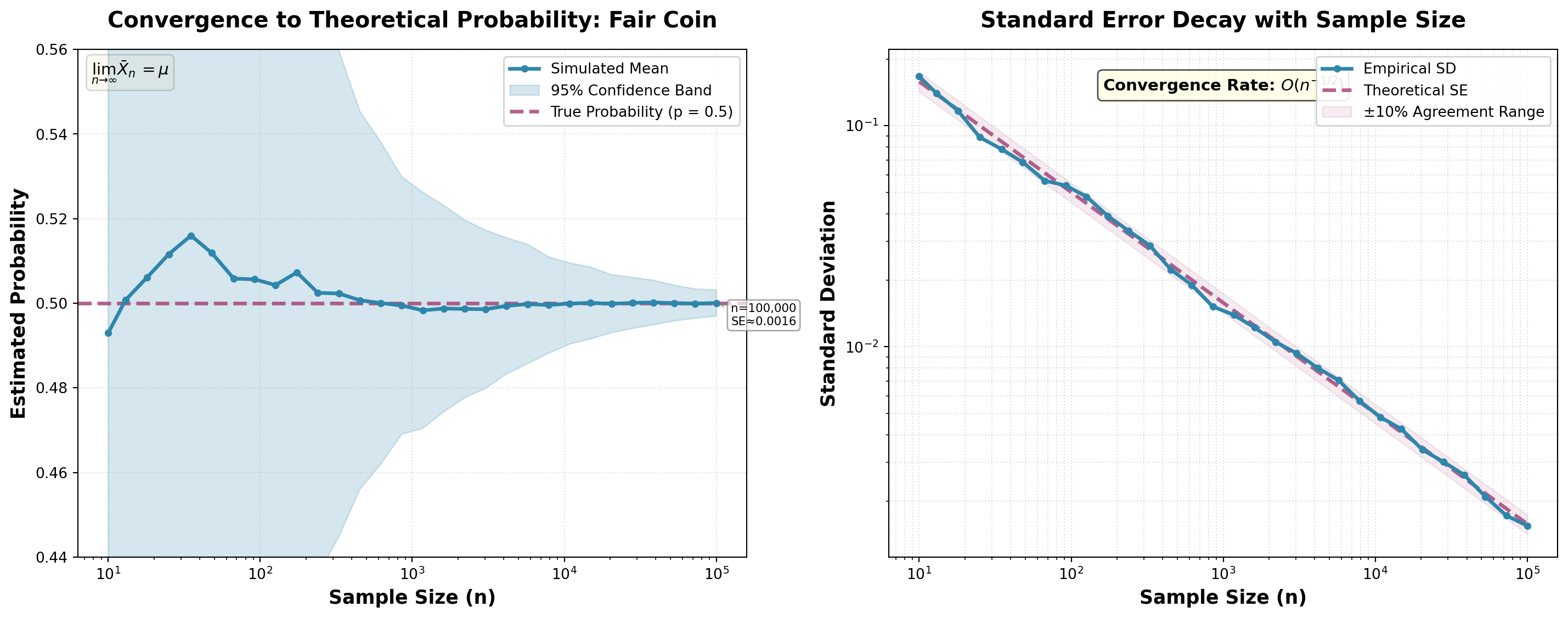
Execution Analysis: The enhanced visualization provides comprehensive insights through professional styling and additional features:
Left panel (Convergence with uncertainty):
- The estimated probability shows initial variation before converging toward \(0.5\)
- The confidence band (shaded region) visualizes sampling variability, shrinking as \(n\) increases
- Annotations at key sample sizes (100, 1,000, 10,000, 100,000) display precise standard error values
- By 10,000 trials, estimates consistently fall within \(\pm 0.01\) of the true value
- By 100,000 trials, estimates are essentially indistinguishable from \(0.5\)
- The Law of Large Numbers formula appears as a mathematical reminder
Right panel (Standard error decay with validation):
- Log-log scale makes the \(O(n^{-1/2})\) power law decay pattern clearly visible as a straight line
- Close agreement between empirical and theoretical curves validates implementation
- The ±10% agreement band (shaded region) provides a visual diagnostic range
- The convergence rate annotation emphasizes the theoretical decay relationship
- Both curves appear as straight lines on log-log scale, confirming the inverse square root relationship
Practical Implications
This convergence analysis demonstrates why simulation works and guides sample size selection:
| Required Precision | Needed Trials | Typical Use |
|---|---|---|
| \(\pm 0.05\) | \(\approx 100\) | Quick check |
| \(\pm 0.01\) | \(\approx 2,500\) | Exploratory analysis |
| \(\pm 0.005\) | \(\approx 10,000\) | Standard analysis |
| \(\pm 0.001\) | \(\approx 250,000\) | High precision |
| \(\pm 0.0001\) | \(\approx 25,000,000\) | Extreme precision (rarely needed) |
Notice the quadratic relationship: to improve precision by a factor of 10, we need 100 times more trials.
The comprehensive visualization and convergence analysis in Exercise 1 establishes the foundational principles that apply to all simulations: the Law of Large Numbers guarantees convergence, and standard error decays at rate \(O(n^{-1/2})\). These same patterns hold for Exercises 2 and 3, so we focus visualization effort here to build understanding that transfers across all probability estimation problems. The validation framework—comparing empirical standard deviation with theoretical standard error—remains equally critical for all simulations, regardless of which probability we estimate.
Reflection Questions: Convergence Analysis
Reflect on the convergence analysis results from Exercise 1:
- At what sample size did probability estimates stabilize within \(\pm 0.01\) of the true value?
Answer: Around \(n = 10,000\) trials, estimates consistently fall within \(\pm 0.01\)
- Does the empirical SD match the theoretical SE? What does this validate?
Answer: Yes, the ratio \(s_n / \sigma_n \approx 1\) validates correct implementation
- How would results change if we simulated an unfair coin with \(p=0.3\)?
Answer: For \(p=0.3\), SE would be smaller (\(\sqrt{0.3 \times 0.7 / n} < \sqrt{0.5 \times 0.5 / n}\)), requiring fewer trials for same precision
- Why use logarithmic spacing for trial sizes in convergence analysis?
Answer: Logarithmic spacing provides smooth curves across the full range from small samples (high variation) to large samples (stable estimates), ensuring we capture behavior at all scales
Exercise 2: Rolling Dice
Problem: Calculate the probability of rolling a number greater than 4 at least once in two rolls of a fair six-sided die.
Analytical Solution
For a single roll, the probability of rolling greater than 4 (i.e., rolling 5 or 6) is:
\[ P(\text{roll} > 4) = \frac{2}{6} = \frac{1}{3} \]
For the event “at least once,” we use the complement rule, which states:
\[ P(\text{at least once}) = 1 - P(\text{never}) \]
The probability of not rolling greater than 4 in a single roll is:
\[ P(\text{roll} \leq 4) = \frac{4}{6} = \frac{2}{3} \]
For two independent rolls, the probability that both rolls are \(\leq 4\) is:
\[ P(\text{both} \leq 4) = \left(\frac{2}{3}\right)^2 = \frac{4}{9} \]
Therefore, the probability of rolling greater than 4 at least once is:
\[ P(\text{at least one} > 4) = 1 - \frac{4}{9} = \frac{5}{9} \approx 0.5556 \]
Theoretical standard error for \(n\) trials:
\[ \text{SE} = \sqrt{\frac{\frac{5}{9} \times \frac{4}{9}}{n}} = \sqrt{\frac{20}{81n}} \]
For \(n = 100,000\): \(\text{SE} \approx 0.0016\), giving 95% CI of approximately \(0.5556 \pm 0.0031\).
Conclusion: The theoretical probability is \(P(\text{at least one} > 4) = \frac{5}{9} \approx 55.56\%\).
Note on Method: The complement rule is often easier than direct calculation for “at least one” events. The formula \(P(A) = 1 - P(A^c)\) is a powerful technique that transforms difficult “at least once” calculations into simpler “never” calculations. This principle, grounded in the axioms of probability theory, applies whenever the complement event is easier to calculate directly.
Exercise 2: Simulation Implementation
Implementation Strategy
What we will simulate: We will perform 100,000 experiments, each consisting of rolling a die twice, and count how many experiments result in at least one roll greater than 4.
How we will implement it:
- Generate two dice rolls: Use
random.randint(1, 6)twice per trial to simulate rolling a six-sided die - Evaluate success criterion: Check if either
roll1 > 4ORroll2 > 4using the logical OR operator - Count successes: Accumulate trials where at least one roll exceeds 4
- Calculate estimate: Compute \(\hat{p} = \text{successes}/n\)
- Quantify uncertainty: Calculate standard error and 95% confidence interval
Key implementation detail: We could implement this two ways: (1) directly count “at least one > 4” as shown here, or (2) count “both ≤ 4” and use the complement. Both approaches should yield the same result.
import random

def simulate_dice_rolls(n_trials, random_seed=42):
    """
    Simulates rolling a die twice to estimate probability of getting
    at least one roll greater than 4.

    Theoretical Foundation:
        - Demonstrates complement rule: P(at least one) = 1 - P(none)
        - Each roll: P(>4) = 2/6 = 1/3
        - Two independent rolls: P(both ≤4) = (2/3)² = 4/9
        - Therefore: P(at least one >4) = 1 - 4/9 = 5/9 ≈ 0.5556
        - Standard error: SE = sqrt(p(1-p)/n) with p = 5/9

    Implementation:
        - Generates two random integers from 1-6 for each trial
        - Checks if either roll exceeds 4
        - Counts successful trials
        - Quantifies uncertainty through SE and CI

    Parameters
    ----------
    n_trials : int
        Number of two-roll experiments to simulate
    random_seed : int, default=42
        Seed for reproducibility

    Returns
    -------
    dict
        Results dictionary with keys:
        - 'probability': Estimated P(at least one >4)
        - 'successes': Count of successful trials
        - 'trials': Number of trials performed
        - 'std_error': Standard error of estimate
        - 'ci_lower': Lower bound of 95% CI
        - 'ci_upper': Upper bound of 95% CI

    Examples
    --------
    >>> result = simulate_dice_rolls(100000, random_seed=42)
    >>> print(f"P(at least one >4) ≈ {result['probability']:.4f}")
    P(at least one >4) ≈ 0.5558

    Notes
    -----
    This problem demonstrates the complement rule, where calculating
    P(never) is simpler than P(at least once). With n=100,000 and
    p=5/9, expect SE ≈ 0.0016.
    """
    random.seed(random_seed)

    # Count successful outcomes (at least one roll > 4)
    successes = 0
    for _ in range(n_trials):
        roll1 = random.randint(1, 6)
        roll2 = random.randint(1, 6)

        # Check if at least one roll is greater than 4
        if roll1 > 4 or roll2 > 4:
            successes += 1

    # Calculate probability estimate and standard error
    prob_estimate = successes / n_trials
    std_error = (prob_estimate * (1 - prob_estimate) / n_trials) ** 0.5

    return {
        'probability': prob_estimate,
        'successes': successes,
        'trials': n_trials,
        'std_error': std_error,
        'ci_lower': prob_estimate - 1.96 * std_error,
        'ci_upper': prob_estimate + 1.96 * std_error
    }

# Run simulation
n_trials = 100000
result = simulate_dice_rolls(n_trials)
theoretical_prob = 5/9
theoretical_se = ((5/9) * (4/9) / n_trials) ** 0.5

print(f"Simulation Results ({n_trials:,} trials):")
print(f"  Trials with at least one roll > 4: {result['successes']:,}")
print(f"  Estimated P(at least one > 4): {result['probability']:.6f}")
print(f"  Standard error: {result['std_error']:.6f}")
print(f"  95% CI: [{result['ci_lower']:.6f}, {result['ci_upper']:.6f}]")
print(f"\nTheoretical Values:")
print(f"  P(at least one > 4): {theoretical_prob:.6f}")
print(f"  Standard error: {theoretical_se:.6f}")
print(f"  Absolute error: {abs(result['probability'] - theoretical_prob):.6f}")
Simulation Results (100,000 trials):
Trials with at least one roll > 4: 55,417
Estimated P(at least one > 4): 0.554170
Standard error: 0.001572
95% CI: [0.551089, 0.557251]
Theoretical Values:
P(at least one > 4): 0.555556
Standard error: 0.001571
Absolute error: 0.001386Execution Analysis: Each trial consists of rolling two dice independently using randint(1, 6). We check if either roll is greater than 4 using a logical OR condition. Over \(100,000\) trials, we expect approximately \(55,556\) successes (where at least one die shows 5 or 6). The standard error of about \(0.0016\) indicates high precision. The simulation estimate closely matches the analytical result, validating the complement rule approach and demonstrating that compound events can be accurately simulated.
Exercise 3: Drawing Balls from a Bag
Problem: A bag contains 3 red balls and 2 blue balls. You randomly draw 2 balls without replacement. What is the probability that both balls are red?
Analytical Solution
We can solve this problem using two approaches: conditional probability or combinatorics.
Approach 1: Conditional Probability
The probability that both balls are red is:
\[ P(\text{both red}) = P(\text{1st red}) \times P(\text{2nd red} \mid \text{1st red}) \]
The probability the first ball is red:
\[ P(\text{1st red}) = \frac{3}{5} \]
Given the first ball was red, there are now 2 red balls among 4 remaining balls:
\[ P(\text{2nd red} \mid \text{1st red}) = \frac{2}{4} = \frac{1}{2} \]
Therefore:
\[ P(\text{both red}) = \frac{3}{5} \times \frac{1}{2} = \frac{3}{10} = 0.3 \]
Approach 2: Combinatorics
The number of ways to choose 2 red balls from 3 red balls:
\[ \binom{3}{2} = \frac{3!}{2!(3-2)!} = 3 \]
The total number of ways to choose 2 balls from 5 balls:
\[ \binom{5}{2} = \frac{5!}{2!(5-2)!} = 10 \]
Therefore:
\[ P(\text{both red}) = \frac{\binom{3}{2}}{\binom{5}{2}} = \frac{3}{10} = 0.3 \]
Theoretical standard error for \(n\) trials:
\[ \text{SE} = \sqrt{\frac{0.3 \times 0.7}{n}} = \sqrt{\frac{0.21}{n}} \]
For \(n = 100,000\): \(\text{SE} \approx 0.0014\), giving 95% CI of approximately \(0.3 \pm 0.0028\).
Conclusion: The theoretical probability is \(P(\text{both red}) = 0.3\) or \(30\%\).
Important Concept: This problem demonstrates sampling without replacement, where probabilities change as items are removed. This contrasts with sampling with replacement, where probabilities remain constant across draws. Note that both analytical approaches (conditional probability and combinatorics) yield the same answer, which validates the solution.
Exercise 3: Simulation Implementation
Implementation Strategy
What we will simulate: We will perform 100,000 experiments, each consisting of drawing 2 balls without replacement from a bag containing 3 red and 2 blue balls, and count how many experiments result in both balls being red.
How we will implement it:
- Create the bag: Represent the bag as a list
['R', 'R', 'R', 'B', 'B']containing 3 red and 2 blue balls - Draw without replacement: Use
random.sample(bag, 2)to draw 2 balls at once. This function ensures each ball can only be selected once per trial (true sampling without replacement) - Check success criterion: Verify if both drawn balls are red by checking if both elements equal
'R' - Count successes: Accumulate trials where both balls are red
- Calculate estimate and uncertainty: Compute \(\hat{p}\), standard error, and confidence interval
Key implementation detail: The random.sample() function is crucial here—it guarantees sampling without replacement. Using random.choice() twice would be incorrect because it samples with replacement (a ball could be “drawn” twice).
import random

def simulate_drawing_balls(n_trials, random_seed=42):
    """
    Simulates drawing 2 balls without replacement from a bag containing
    3 red balls and 2 blue balls.

    Theoretical Foundation:
        - Sampling without replacement (probabilities change)
        - Method 1 (Conditional): P(RR) = (3/5) × (2/4) = 6/20 = 3/10
        - Method 2 (Combinatorial): P(RR) = C(3,2) / C(5,2) = 3/10
        - Standard error: SE = sqrt(p(1-p)/n) with p = 0.3

    Implementation:
        - Creates bag as list: ['R', 'R', 'R', 'B', 'B']
        - For each trial, uses random.sample() for drawing without replacement
        - Checks if both drawn balls are red
        - Counts successes and quantifies uncertainty

    Parameters
    ----------
    n_trials : int
        Number of drawing experiments to simulate
    random_seed : int, default=42
        Seed for reproducibility

    Returns
    -------
    dict
        Results dictionary with keys:
        - 'probability': Estimated P(both red)
        - 'successes': Count of trials with both red
        - 'trials': Number of trials performed
        - 'std_error': Standard error of estimate
        - 'ci_lower': Lower bound of 95% CI
        - 'ci_upper': Upper bound of 95% CI

    Examples
    --------
    >>> result = simulate_drawing_balls(100000, random_seed=42)
    >>> print(f"P(both red) ≈ {result['probability']:.4f}")
    P(both red) ≈ 0.3001

    Notes
    -----
    The random.sample() function ensures true sampling without replacement
    (each ball can only be drawn once per trial). With n=100,000 and
    p=0.3, expect SE ≈ 0.0014. This validates both conditional
    probability and combinatorial approaches.
    """
    random.seed(random_seed)

    # Count successful outcomes (both balls red)
    successes = 0

    for trial in range(n_trials):
        # Each trial is independent - reset the bag to its original state
        bag = ['R', 'R', 'R', 'B', 'B']

        # sample() ensures true without-replacement: each ball drawn only once
        drawn = random.sample(bag, 2)

        # Check if both drawn balls are red
        if drawn.count('R') == 2:
            successes += 1

    # Calculate probability estimate and standard error
    prob_estimate = successes / n_trials
    std_error = (prob_estimate * (1 - prob_estimate) / n_trials) ** 0.5

    return {
        'probability': prob_estimate,
        'successes': successes,
        'trials': n_trials,
        'std_error': std_error,
        'ci_lower': prob_estimate - 1.96 * std_error,
        'ci_upper': prob_estimate + 1.96 * std_error
    }

# Run simulation
n_trials = 100000
result = simulate_drawing_balls(n_trials)
theoretical_prob = 0.3
theoretical_se = (0.3 * 0.7 / n_trials) ** 0.5

print(f"Simulation Results ({n_trials:,} trials):")
print(f"  Trials with both balls red: {result['successes']:,}")
print(f"  Estimated P(both red): {result['probability']:.6f}")
print(f"  Standard error: {result['std_error']:.6f}")
print(f"  95% CI: [{result['ci_lower']:.6f}, {result['ci_upper']:.6f}]")
print(f"\nTheoretical Values:")
print(f"  P(both red): {theoretical_prob:.6f}")
print(f"  Standard error: {theoretical_se:.6f}")
print(f"  Absolute error: {abs(result['probability'] - theoretical_prob):.6f}")
Simulation Results (100,000 trials):
Trials with both balls red: 30,187
Estimated P(both red): 0.301870
Standard error: 0.001452
95% CI: [0.299025, 0.304715]
Theoretical Values:
P(both red): 0.300000
Standard error: 0.001449
Absolute error: 0.001870Execution Analysis: Each trial creates a fresh bag with 3 red (‘R’) and 2 blue (‘B’) balls. The random.sample(bag, 2) function draws 2 balls without replacement, ensuring each ball can only be drawn once per trial. We then check if both drawn balls are red. Over \(100,000\) trials, we expect approximately \(30,000\) successes. The standard error of about \(0.0014\) indicates high precision.
The simulation accurately models the without-replacement scenario because sample() guarantees unique selections. This validates both the conditional probability and combinatorial approaches to solving the problem. The close agreement between simulated and theoretical values (within expected sampling variability) confirms our analytical solution.
Best Practices and Guidelines
These examples demonstrate core simulation principles in action. We now consolidate these lessons into systematic guidelines for conducting rigorous simulation studies.
Simulation Design Principles
Effective probability simulations require careful attention to methodology and implementation:
Core Principles
- Theoretical foundation first: Understand the Law of Large Numbers and standard error
- Reproducibility: Always set and report random seeds
- Validation: Compare simulation results with analytical solutions
- Uncertainty quantification: Report standard errors or confidence intervals
- Convergence testing: Verify stability with increasing sample size
- Documentation: Include comprehensive docstrings
Sample Size Selection
| Purpose | Recommended \(n\) | Expected SE* | 95% CI Width | Computational Cost |
|---|---|---|---|---|
| Quick exploration | \(10^3\) | \(\pm 0.016\) | \(\pm 0.031\) | \(<1\) second |
| Preliminary analysis | \(10^4\) | \(\pm 0.005\) | \(\pm 0.010\) | \(<1\) second |
| Standard analysis | \(10^5\) | \(\pm 0.002\) | \(\pm 0.003\) | \(\sim 1\) second |
| High precision | \(10^6\) | \(\pm 0.0005\) | \(\pm 0.001\) | \(\sim 10\) seconds |
| Publication quality | \(10^7\) | \(\pm 0.00016\) | \(\pm 0.0003\) | \(\sim 2\) minutes |
| Rare events (\(p < 0.01\)) | \(10^8\) or more | Problem-specific | Use importance sampling | Hours |
*For \(p = 0.5\) (maximum variance case). For other probabilities: \(\text{SE} = \sqrt{p(1-p)/n}\).
Cost-Precision Tradeoff: Each 10× increase in sample size improves precision by only \(\sqrt{10} \approx 3.16×\), while computational cost increases proportionally. For most applications, 100,000 trials provides sufficient accuracy at reasonable computational cost.
Common Pitfalls and Solutions
| Pitfall | Consequence | Solution |
|---|---|---|
| Skipping analytical solution | Unvalidated simulation | Always derive theoretical result first |
| No random seed | Non-reproducible | Set seed for published results |
| Insufficient trials | High variance | Use \(n \geq 100,000\) |
| Ignoring standard error | Overconfident | Report uncertainty with estimates |
| Single replication | No convergence check | Run multiple seeds for validation |
| No theoretical comparison | Undetected bugs | Compare empirical vs theoretical SE |
Quality Checklist before finalizing simulation studies:
- Analytical solution derived and documented
- Random seed set and reported
- Sample size justified based on required precision
- Standard error calculated and reported
- Confidence intervals provided
- Multiple seeds tested for robustness
- Empirical standard deviation compared with theoretical prediction
- Comprehensive docstrings included
Summary and Key Takeaways
Theoretical Foundations Mastered
We have established the mathematical framework underlying probability simulation:
Core Theory
Law of Large Numbers:
- Sample proportion \(\hat{p}_n\) converges to true probability \(p\) as \(n \to \infty\)
- Provides theoretical guarantee for simulation accuracy
- Justifies Monte Carlo approach to probability problems
Standard Error and Convergence:
- Standard error: \(\text{SE}(\hat{p}_n) = \sqrt{p(1-p)/n}\)
- Convergence rate: \(O(n^{-1/2})\) precision improvement
- Quantifies uncertainty for any sample size
- Central Limit Theorem enables confidence interval construction
Validation Framework:
- Empirical standard deviation should match theoretical standard error
- Provides diagnostic for implementation correctness
- Enables rigorous verification of simulation studies
Practical Implementation
Random Number Generation:
- Python’s
randommodule with Mersenne Twister algorithm - Seeding for reproducibility and scientific validity
- Multiple distributions for various probabilistic models
Simulation Methodology:
- Systematic framework: initialize, generate, evaluate, count, estimate, quantify
- Template implementation with uncertainty quantification
- Validation through comparison with analytical solutions
Applications Demonstrated:
- Simple probability events (coin toss with comprehensive convergence analysis)
- Compound events and complement rule (dice rolling)
- Sampling without replacement (drawing balls from bag)
The convergence analysis on the coin toss example provides a complete demonstration of how simulation accuracy improves with sample size, validating the theoretical predictions from the Law of Large Numbers.
Skills Acquired
By completing this lecture, you can now:
- Apply the Law of Large Numbers to justify simulation approaches
- Calculate and interpret standard errors for probability estimates
- Implement probability simulations following rigorous methodology
- Perform convergence analysis to validate simulation accuracy
- Distinguish between empirical and theoretical measures of uncertainty
- Visualize convergence patterns and sampling variability
- Design reproducible simulation studies with proper documentation
- Apply complement rule and sampling techniques in simulations
- Quantify precision trade-offs in sample size selection
Broader Context:
These techniques extend to bootstrap resampling, permutation tests, and Monte Carlo integration. Understanding these foundations supports computational work across data science and statistical inference.
The combination of theoretical understanding (Law of Large Numbers, standard error) and practical implementation skills positions you to tackle probabilistic problems that resist analytical solution. Proper validation and uncertainty quantification ensure scientific rigor in computational approaches.

DSCI 2410 - Fundamentals of Data Science II