Counting Principles

Permutations, Combinations, and Combinatorial Analysis

Ahmed Moustafa

amoustafa@aucegypt.edu

The American University in Cairo

2025-10-29

Learning Objectives

By the end of this lecture, you will be able to:

Core Concepts:

• Understand and apply the fundamental counting principle
• Use factorial notation to solve arrangement problems
• Distinguish between permutations and combinations
• Solve ordering problems with and without replacement

Advanced Techniques:

• Calculate permutations of subsets: \(P(n,k)\)
• Determine combinations without regard to order: \(\binom{n}{k}\)
• Solve counting problems with constraints
• Handle indistinguishable objects and repetition cases

Success Criteria: You will solve real-world counting problems by selecting appropriate combinatorial techniques and justifying your mathematical approach.

Introduction to Counting Principles

Combinatorics is the branch of mathematics concerned with counting, arranging, and selecting objects. These principles form the foundation for probability theory, statistics, and computational complexity analysis.

Efficient counting methods are fundamental to data science, enabling us to:

• Determine the number of possible outcomes in sample spaces
• Analyze algorithm complexity and computational feasibility
• Design experiments and sample surveys
• Understand combinatorial structures in data

Historical Context

The formal study of combinatorics began in the 17th century with Blaise Pascal and Pierre de Fermat, who developed the foundations of probability theory through correspondence about gambling problems in 1654.

The notation for combinations, \(\binom{n}{k}\), appeared in Pascal’s Traité du triangle arithmétique (1665), which introduced Pascal’s triangle and established the mathematical framework for binomial coefficients.

Why Counting Matters

Counting principles enable us to:

• Quantify possibilities in decision-making scenarios
• Determine favorable outcomes in various scenarios
• Analyze complexity of algorithms and data structures
• Design experiments by understanding sample space size
• Solve optimization problems through enumeration

Data Science Applications

Counting principles appear throughout data science practice in several contexts:

Feature Engineering: With \(5\) categorical variables, each having \(10\) levels, interaction features generate \(10^5 = 100,000\) possible combinations, requiring computational consideration.

Permutation Testing: Computing exact \(p\)-values requires counting all possible rearrangements of observed data to establish the null distribution.

Hyperparameter Optimization: A grid search over \(5\) hyperparameters with \(10\) values each examines \(10^5\) configurations, making the search space size critical for feasibility.

Experimental Design: Determining valid treatment assignments in randomized trials depends on combinatorial analysis to ensure proper randomization.

Model Selection: With multiple feature engineering options, cross-validation strategies, and hyperparameter choices, the combinatorial explosion requires systematic enumeration.

Without systematic counting methods, exhaustive enumeration becomes impractical. An \(8\)-character alphanumeric password has \(62^8 \approx 2.18 \times 10^{14}\) possibilities. In genomics, enumerating all \(k\)-mer sequences of length \(20\) from DNA yields \(4^{20} \approx 1.1 \times 10^{12}\) combinations, which is computationally prohibitive.

The Fundamental Counting Principle

graph TB
    A["Fundamental Counting Principle"] --> B["Task 1<br/>m choices"]
    A --> C["Task 2<br/>n choices"]
    A --> D["Task 3<br/>p choices"]
    
    B --> E["Total Ways"]
    C --> E
    D --> E
    
    E --> F["m × n × p"]
    
    style A fill:#2E7D32,color:#FFFFFF
    style B fill:#1565C0,color:#FFFFFF
    style C fill:#1565C0,color:#FFFFFF
    style D fill:#1565C0,color:#FFFFFF
    style E fill:#E65100,color:#FFFFFF
    style F fill:#6A1B9A,color:#FFFFFF

Principle: If a task can be performed in \(m\) ways, and for each of these ways a second task can be performed in \(n\) ways, then the two tasks together can be performed in \(m \times n\) ways.

This generalizes to any number of sequential tasks: if tasks have \(m_1, m_2, \ldots, m_k\) choices respectively, the total number of ways to complete all tasks is:

\[ \prod_{i=1}^{k} m_i = m_1 \times m_2 \times \cdots \times m_k \]

Factorials

Factorial Notation

The factorial of a non-negative integer \(n\), denoted \(n!\), is the product of all positive integers less than or equal to \(n\).

Mathematical Definition

\[ n! = \begin{cases} 1 & \text{if } n = 0 \\ n \times (n-1) \times (n-2) \times \cdots \times 2 \times 1 & \text{if } n > 0 \end{cases} \]

Equivalently, we can define factorials recursively:

\[ n! = \begin{cases} 1 & \text{if } n = 0 \\ n \times (n-1)! & \text{if } n > 0 \end{cases} \]

Interpretation: The value \(n!\) represents the number of ways to arrange \(n\) distinct objects in a sequence.

Python Modules and Importing

Before we begin working with factorials computationally, we need to understand how to access Python’s built-in mathematical functions through modules.

What is a Module?

A module is a file containing Python definitions and statements. Python organizes its standard library into modules to group related functionality together. This organizational approach:

• Keeps the core language clean and efficient
• Allows you to load only the functions you need
• Prevents naming conflicts between different functions
• Enables code reuse across projects

Think of modules as toolboxes. Python comes with many toolboxes (modules), each containing specialized tools (functions). The math module, for instance, contains mathematical functions beyond basic arithmetic.

Importing Modules

To use functions from a module, you must first import the module using the import statement:

import math

# Now we can use math module functions
result_5 = math.factorial(5)
result_10 = math.factorial(10)

print(f"5! = {result_5}")
print(f"10! = {result_10}")

5! = 120
10! = 3628800

Alternative Import Syntax

Python offers several ways to import modules:

# Method 1: Import entire module
import math
value1 = math.factorial(6)

# Method 2: Import specific function
from math import factorial
value2 = factorial(6)

# Method 3: Import with alias
import math as m
value3 = m.factorial(6)

print(f"Method 1: {value1}")
print(f"Method 2: {value2}")
print(f"Method 3: {value3}")

Method 1: 720
Method 2: 720
Method 3: 720

Best Practice: For standard modules like math, use import math rather than from math import *. This makes your code more readable by clearly showing where functions come from.

Computing Factorials

Manual Implementation

Understanding how factorials are computed helps build computational thinking:

def factorial_iterative(n):
    """
    Calculate factorial using iterative approach.
    
    Args:
        n (int): Non-negative integer
        
    Returns:
        int: n!
    """
    if n < 0:
        raise ValueError("Factorial not defined for negative numbers")
    
    result = 1
    for i in range(2, n + 1):
        result *= i
    
    return result

# Test the implementation
for n in range(8):
    print(f"{n}! = {factorial_iterative(n):,}")

0! = 1
1! = 1
2! = 2
3! = 6
4! = 24
5! = 120
6! = 720
7! = 5,040

Recursive Implementation

The recursive definition translates directly into code:

def factorial_recursive(n):
    """
    Calculate factorial using recursion.
    
    Args:
        n (int): Non-negative integer
        
    Returns:
        int: n!
    """
    if n < 0:
        raise ValueError("Factorial not defined for negative numbers")
    
    # Base cases
    if n == 0 or n == 1:
        return 1
    
    # Recursive case
    return n * factorial_recursive(n - 1)

# Test recursive implementation
print("Recursive factorial:")
for n in range(8):
    print(f"{n}! = {factorial_recursive(n):,}")

Recursive factorial:
0! = 1
1! = 1
2! = 2
3! = 6
4! = 24
5! = 120
6! = 720
7! = 5,040

Comparing Implementations

import time

def time_factorial_methods(n):
    """Compare execution time of different factorial methods."""
    
    # Built-in method
    start = time.time()
    result_builtin = math.factorial(n)
    time_builtin = time.time() - start
    
    # Iterative method
    start = time.time()
    result_iterative = factorial_iterative(n)
    time_iterative = time.time() - start
    
    # Recursive method (careful with large n)
    if n < 1000:  # Avoid recursion limit
        start = time.time()
        result_recursive = factorial_recursive(n)
        time_recursive = time.time() - start
    else:
        result_recursive = "N/A"
        time_recursive = float('inf')
    
    print(f"\nFactorial of {n}:")
    print(f"  Built-in:   {time_builtin:.6f} seconds")
    print(f"  Iterative:  {time_iterative:.6f} seconds")
    if n < 1000:
        print(f"  Recursive:  {time_recursive:.6f} seconds")

# Compare methods
time_factorial_methods(100)
time_factorial_methods(500)

Factorial of 100:
  Built-in:   0.000002 seconds
  Iterative:  0.000005 seconds
  Recursive:  0.000007 seconds

Factorial of 500:
  Built-in:   0.000009 seconds
  Iterative:  0.000048 seconds
  Recursive:  0.000076 seconds

The built-in math.factorial() is implemented in C and optimized for performance. For production code, always use the built-in implementation. Manual implementations are valuable for understanding the underlying algorithm. Note that Python’s default recursion limit is approximately 1000, so recursive factorial will raise RecursionError for \(n > 1000\).

Example: Arranging Books

Problem: In how many ways can you arrange 5 different books on a shelf?

Solution:

We need to determine the number of distinct orderings of 5 books.

Step 1: Identify the problem type
This is an arrangement problem where all objects are distinct and order matters.

Step 2: Apply the counting principle
For each position on the shelf, we have a decreasing number of choices:

• First position: 5 choices (any of the 5 books)
• Second position: 4 remaining choices
• Third position: 3 remaining choices
• Fourth position: 2 remaining choices
• Fifth position: 1 remaining choice

Step 3: Calculate the total
By the multiplication principle:

\[ 5 \times 4 \times 3 \times 2 \times 1 = 5! = 120 \text{ ways} \]

Step 4: Verify computationally

num_books = 5
arrangements = math.factorial(num_books)

print(f"Number of ways to arrange {num_books} books: {arrangements}")

# Verify with all arrangements for 3 books
from itertools import permutations

books = ['A', 'B', 'C']
all_arrangements = list(permutations(books))

print(f"\nFor {len(books)} books, there are {math.factorial(len(books))} arrangements:")
for i, arrangement in enumerate(all_arrangements, 1):
    print(f"  {i}. {' '.join(arrangement)}")

Number of ways to arrange 5 books: 120

For 3 books, there are 6 arrangements:
  1. A B C
  2. A C B
  3. B A C
  4. B C A
  5. C A B
  6. C B A

Answer: There are 120 distinct ways to arrange 5 different books on a shelf.

Factorial Growth

Factorials grow extremely rapidly, faster than exponential functions. This rapid growth has important implications for computational complexity and algorithm design.

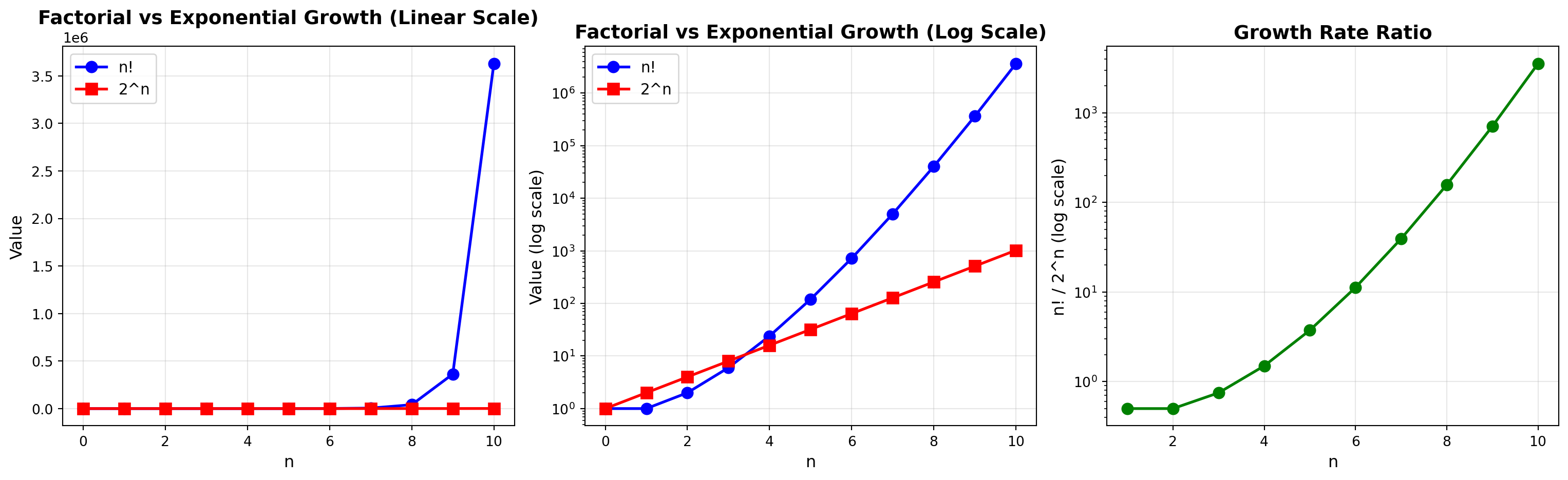
Factorial vs Exponential Growth Comparison:
n     n!                   2^n                  n!/2^n               Scientific          
------------------------------------------------------------------------------------------
0     1                    1                    1.00                 1.00e+00            
1     1                    2                    0.50                 1.00e+00            
2     2                    4                    0.50                 2.00e+00            
3     6                    8                    0.75                 6.00e+00            
4     24                   16                   1.50                 2.40e+01            
5     120                  32                   3.75                 1.20e+02            
6     720                  64                   11.25                7.20e+02            
7     5,040                128                  39.38                5.04e+03            
8     40,320               256                  157.50               4.03e+04            
9     362,880              512                  708.75               3.63e+05            
10    3,628,800            1,024                3543.75              3.63e+06            
11    39,916,800           2,048                19490.62             3.99e+07            
12    479,001,600          4,096                116943.75            4.79e+08            
13    6,227,020,800        8,192                760134.38            6.23e+09            
14    87,178,291,200       16,384               5320940.62           8.72e+10            
15    1,307,674,368,000    32,768               39907054.69          1.31e+12            

Key Observation: Factorial growth eventually dominates exponential growth.
At n=10: 10! / 2^10 = 3543.75
At n=15: 15! / 2^15 = 39907054.69

Note that \(20! = 2,432,902,008,176,640,000\) is already beyond what can be stored in standard 64-bit integers in many programming languages. Python handles arbitrary precision integers natively, but this comes with performance costs. The rapid growth of factorials explains why exhaustive search algorithms become infeasible quickly. Even modest values of \(n\) create astronomical numbers of possibilities.

Permutations

Definition and Notation

A permutation is an ordered arrangement of objects. When we care about the order in which objects appear, we use permutations.

Notation: The number of ways to arrange \(k\) objects selected from \(n\) distinct objects is denoted \(P(n,k)\) or \(_nP_k\) or \(^nP_k\).

Formula

\[ P(n,k) = \frac{n!}{(n-k)!} \]

This formula can be understood through the fundamental counting principle:

• First position: \(n\) choices
• Second position: \(n-1\) choices (one already selected)
• Third position: \(n-2\) choices
• …
• \(k\)-th position: \(n-k+1\) choices

Therefore:

\[ P(n,k) = n \times (n-1) \times (n-2) \times \cdots \times (n-k+1) = \frac{n!}{(n-k)!} \]

Special Case

When \(k = n\) (arranging all \(n\) objects):

\[ P(n,n) = \frac{n!}{(n-n)!} = \frac{n!}{0!} = \frac{n!}{1} = n! \]

Computing Permutations in Python

Python provides math.perm() for computing permutations (available in Python 3.8+):

# Using Python's built-in function
n, k = 10, 3
result = math.perm(n, k)

print(f"P({n},{k}) = {result}")

# Verify with formula
result_formula = math.factorial(n) // math.factorial(n - k)
print(f"Using formula: {result_formula}")
print(f"Match: {result == result_formula}")

# Examples
print("\nPermutation examples:")
for n_val, k_val in [(5, 2), (8, 3), (10, 4), (7, 7)]:
    perm_value = math.perm(n_val, k_val)
    print(f"  P({n_val},{k_val}) = {perm_value:,}")

P(10,3) = 720
Using formula: 720
Match: True

Permutation examples:
  P(5,2) = 20
  P(8,3) = 336
  P(10,4) = 5,040
  P(7,7) = 5,040

Example: Password Creation

Problem: How many 4-character passwords can be formed from 26 lowercase letters if no letter can be repeated?

Solution:

Step 1: Identify the problem type
This is a permutation problem because:

• We are selecting 4 letters from 26 available letters
• Order matters (the password “abcd” is different from “dcba”)
• No repetition is allowed (each letter used once)

Step 2: Define parameters
- Total letters available: \(n = 26\) - Password length: \(k = 4\)

Step 3: Apply the permutation formula

\[ P(26, 4) = \frac{26!}{(26-4)!} = \frac{26!}{22!} \]

Step 4: Calculate
The factorials simplify to:

\[ P(26, 4) = 26 \times 25 \times 24 \times 23 = 358,800 \]

Step 5: Verify computationally

n_letters = 26
password_length = 4

num_passwords = math.perm(n_letters, password_length)

print(f"Number of {password_length}-character passwords (no repetition): {num_passwords:,}")

# Manual calculation for verification
manual_calc = 26 * 25 * 24 * 23
print(f"Manual calculation: {manual_calc:,}")
print(f"Match: {num_passwords == manual_calc}")

# Compare with repetition allowed
with_repetition = n_letters ** password_length
print(f"\nWith repetition allowed: {with_repetition:,}")
print(f"Increase factor: {with_repetition / num_passwords:.2f}x")

Number of 4-character passwords (no repetition): 358,800
Manual calculation: 358,800
Match: True

With repetition allowed: 456,976
Increase factor: 1.27x

Answer: There are 358,800 distinct 4-character passwords that can be formed from 26 lowercase letters without repetition.

For comparison, if repetition were allowed, the number would increase to \(26^4 = 456,976\) passwords, representing a 1.27x increase.

Example: Race Podium

Problem: In a race with 12 runners, how many different ways can the gold, silver, and bronze medals be awarded?

Solution:

Step 1: Identify the problem type
This is a permutation problem because:

• We select 3 runners from 12
• Order matters (gold, silver, bronze are distinct positions)
• No repetition (one runner cannot receive multiple medals)

Step 2: Define parameters
- Total runners: \(n = 12\) - Medals to award: \(k = 3\)

Step 3: Apply the formula

\[ P(12, 3) = \frac{12!}{(12-3)!} = \frac{12!}{9!} = 12 \times 11 \times 10 = 1,320 \]

Step 4: Verify computationally

runners = 12
medals = 3

podium_arrangements = math.perm(runners, medals)

print(f"Number of possible podium arrangements: {podium_arrangements:,}")

# Simulate small example with 4 runners
from itertools import permutations

runners_small = ['A', 'B', 'C', 'D']
podium_small = list(permutations(runners_small, 3))

print(f"\nFor {len(runners_small)} runners and 3 medals:")
print(f"Calculated: P({len(runners_small)}, 3) = {math.perm(len(runners_small), 3)}")
print(f"Enumerated: {len(podium_small)} arrangements")
print("\nFirst 10 arrangements:")
for i, arrangement in enumerate(podium_small[:10], 1):
    print(f"  {i}. Gold: {arrangement[0]}, Silver: {arrangement[1]}, Bronze: {arrangement[2]}")

Number of possible podium arrangements: 1,320

For 4 runners and 3 medals:
Calculated: P(4, 3) = 24
Enumerated: 24 arrangements

First 10 arrangements:
  1. Gold: A, Silver: B, Bronze: C
  2. Gold: A, Silver: B, Bronze: D
  3. Gold: A, Silver: C, Bronze: B
  4. Gold: A, Silver: C, Bronze: D
  5. Gold: A, Silver: D, Bronze: B
  6. Gold: A, Silver: D, Bronze: C
  7. Gold: B, Silver: A, Bronze: C
  8. Gold: B, Silver: A, Bronze: D
  9. Gold: B, Silver: C, Bronze: A
  10. Gold: B, Silver: C, Bronze: D

Answer: There are 1,320 different ways to award the gold, silver, and bronze medals among 12 runners.

Note that if we only cared about which 3 runners received medals (not their specific ranks), we would use combinations instead, which would give us \(\binom{12}{3} = 220\) possibilities.

Permutations with Repetition

When objects are not all distinct, we must account for indistinguishable arrangements.

Formula: If we have \(n\) objects where \(n_1\) are of type 1, \(n_2\) are of type 2, …, and \(n_k\) are of type \(k\), the number of distinct permutations is:

\[ \frac{n!}{n_1! \cdot n_2! \cdot \ldots \cdot n_k!} \]

We divide by the factorials of repeated elements because swapping identical objects produces the same arrangement.

Example: Anagrams

Problem: How many distinct arrangements can be made from the letters in “MISSISSIPPI”?

Solution:

Step 1: Count the letters
- Total letters: \(n = 11\) - Letter frequencies:

• M: 1
• I: 4
• S: 4
• P: 2

Step 2: Identify the problem type
This is a permutation with repetition problem because we have identical letters that are indistinguishable from each other.

Step 3: Apply the formula
For permutations with repetition:

\[ \frac{n!}{n_1! \cdot n_2! \cdot n_3! \cdot n_4!} = \frac{11!}{1! \cdot 4! \cdot 4! \cdot 2!} \]

Step 4: Calculate

\[ \frac{11!}{1! \cdot 4! \cdot 4! \cdot 2!} = \frac{39,916,800}{1 \cdot 24 \cdot 24 \cdot 2} = \frac{39,916,800}{1,152} = 34,650 \]

Step 5: Verify computationally

from collections import Counter

word = "MISSISSIPPI"
n = len(word)

# Count letter frequencies
letter_counts = Counter(word)

# Calculate distinct arrangements
numerator = math.factorial(n)
denominator = 1
for count in letter_counts.values():
    denominator *= math.factorial(count)

distinct_arrangements = numerator // denominator

print(f"Word: {word}")
print(f"Total letters: {n}")
print(f"Letter frequencies: {dict(letter_counts)}")
print(f"\nDistinct arrangements: {distinct_arrangements:,}")
print(f"\nCalculation:")
print(f"  Numerator (11!): {numerator:,}")
print(f"  Denominator (1! × 4! × 4! × 2!): {denominator:,}")

Word: MISSISSIPPI
Total letters: 11
Letter frequencies: {'M': 1, 'I': 4, 'S': 4, 'P': 2}

Distinct arrangements: 34,650

Calculation:
  Numerator (11!): 39,916,800
  Denominator (1! × 4! × 4! × 2!): 1,152

Answer: There are 34,650 distinct arrangements of the letters in “MISSISSIPPI”.

The division by the factorials of repeated letters accounts for the fact that swapping identical letters (e.g., swapping two I’s or two S’s) produces the same arrangement.

Combinations

Definition and Notation

A combination is a selection of objects where order does not matter. When we only care about which objects are selected (not their arrangement), we use combinations.

Notation: The number of ways to select \(k\) objects from \(n\) distinct objects is denoted \(\binom{n}{k}\) (read as “n choose k”) or \(C(n,k)\) or \(_nC_k\).

Formula

\[ \binom{n}{k} = \frac{n!}{k!(n-k)!} \]

This formula follows from the relationship between permutations and combinations:

\[ \binom{n}{k} = \frac{P(n,k)}{k!} = \frac{n!/(n-k)!}{k!} = \frac{n!}{k!(n-k)!} \]

We divide by \(k!\) because the \(k!\) different orderings of the selected objects all represent the same combination.

Relationship Between Permutations and Combinations

The key relationship between permutations and combinations is:

\[ P(n,k) = \binom{n}{k} \times k! \]

Reasoning:

1. When we select \(k\) objects from \(n\) objects without regard to order, we get \(\binom{n}{k}\) combinations
2. Each of these combinations can be arranged in \(k!\) different ways
3. Therefore, the total number of permutations equals the number of combinations multiplied by the number of ways to arrange each combination

Solving for combinations:

\[ \binom{n}{k} = \frac{P(n,k)}{k!} = \frac{n!/(n-k)!}{k!} = \frac{n!}{k!(n-k)!} \]

This explains why we divide by \(k!\) when computing combinations: we are removing the \(k!\) different orderings that all represent the same selection.

Computing Combinations in Python

Python provides math.comb() for computing combinations:

# Using Python's built-in function
n, k = 10, 3
result = math.comb(n, k)

print(f"C({n},{k}) = {result}")

# Verify with formula
result_formula = math.factorial(n) // (math.factorial(k) * math.factorial(n - k))
print(f"Using formula: {result_formula}")
print(f"Match: {result == result_formula}")

# Verify relationship with permutations
perm_value = math.perm(n, k)
factorial_k = math.factorial(k)
comb_from_perm = perm_value // factorial_k

print(f"\nVerifying P(n,k) = C(n,k) × k!:")
print(f"  P({n},{k}) = {perm_value}")
print(f"  C({n},{k}) = {result}")
print(f"  k! = {factorial_k}")
print(f"  P({n},{k}) / k! = {comb_from_perm}")
print(f"  Match: {result == comb_from_perm}")

C(10,3) = 120
Using formula: 120
Match: True

Verifying P(n,k) = C(n,k) × k!:
  P(10,3) = 720
  C(10,3) = 120
  k! = 6
  P(10,3) / k! = 120
  Match: True

Example: Committee Selection

Problem: From a group of 10 people, how many ways can we select a committee of 4?

Solution:

Step 1: Identify the problem type
This is a combination problem because:

• We are selecting 4 people from 10
• Order does not matter (the committee {A, B, C, D} is the same as {D, C, B, A})
• No repetition (each person selected once)

Step 2: Define parameters
- Total people: \(n = 10\) - Committee size: \(k = 4\)

Step 3: Apply the formula

\[ \binom{10}{4} = \frac{10!}{4! \cdot 6!} \]

Step 4: Simplify the calculation
Rather than computing full factorials, we can simplify:

\[ \binom{10}{4} = \frac{10 \times 9 \times 8 \times 7}{4 \times 3 \times 2 \times 1} = \frac{5,040}{24} = 210 \]

Step 5: Verify computationally

n_people = 10
committee_size = 4

num_committees = math.comb(n_people, committee_size)

print(f"Number of possible {committee_size}-person committees from {n_people} people: {num_committees}")

# Manual calculation
numerator = n_people * 9 * 8 * 7
denominator = 4 * 3 * 2 * 1
manual_result = numerator // denominator

print(f"\nManual calculation:")
print(f"  Numerator: {n_people} × 9 × 8 × 7 = {numerator:,}")
print(f"  Denominator: 4 × 3 × 2 × 1 = {denominator}")
print(f"  Result: {manual_result}")

# Show small example
from itertools import combinations

people = ['A', 'B', 'C', 'D', 'E']
committees_small = list(combinations(people, 3))

print(f"\nExample: {len(committees_small)} committees of 3 from 5 people:")
for i, committee in enumerate(committees_small, 1):
    print(f"  {i}. {{{', '.join(committee)}}}")

Number of possible 4-person committees from 10 people: 210

Manual calculation:
  Numerator: 10 × 9 × 8 × 7 = 5,040
  Denominator: 4 × 3 × 2 × 1 = 24
  Result: 210

Example: 10 committees of 3 from 5 people:
  1. {A, B, C}
  2. {A, B, D}
  3. {A, B, E}
  4. {A, C, D}
  5. {A, C, E}
  6. {A, D, E}
  7. {B, C, D}
  8. {B, C, E}
  9. {B, D, E}
  10. {C, D, E}

Answer: There are 210 different ways to select a 4-person committee from 10 people.

Example: Poker Hand

Problem: How many different 5-card poker hands can be dealt from a standard 52-card deck?

Solution:

Step 1: Identify the problem type
This is a combination problem because:

• We select 5 cards from 52
• Order does not matter (a hand is defined by which cards it contains, not their order)

Step 2: Apply the formula

\[ \binom{52}{5} = \frac{52!}{5! \cdot 47!} \]

Step 3: Calculate

\[ \binom{52}{5} = \frac{52 \times 51 \times 50 \times 49 \times 48}{5 \times 4 \times 3 \times 2 \times 1} = \frac{311,875,200}{120} = 2,598,960 \]

Step 4: Verify and explore

deck_size = 52
hand_size = 5

num_hands = math.comb(deck_size, hand_size)

print(f"Number of possible {hand_size}-card hands from {deck_size} cards: {num_hands:,}")

# Compare with permutations
if_order_mattered = math.perm(deck_size, hand_size)
print(f"\nIf order mattered: {if_order_mattered:,}")
print(f"Reduction factor: {if_order_mattered / num_hands:.0f}x (which is {hand_size}!)")

# Probability of specific hand types
royal_flush_count = 4  # One per suit
royal_flush_prob = royal_flush_count / num_hands

print(f"\nProbability of royal flush: {royal_flush_prob:.10f}")
print(f"Or approximately 1 in {num_hands / royal_flush_count:,.0f}")

Number of possible 5-card hands from 52 cards: 2,598,960

If order mattered: 311,875,200
Reduction factor: 120x (which is 5!)

Probability of royal flush: 0.0000015391
Or approximately 1 in 649,740

Answer: There are 2,598,960 distinct 5-card poker hands possible from a standard 52-card deck.

The probability of being dealt a royal flush (10, J, Q, K, A of the same suit) is approximately 1 in 649,740, demonstrating why it is the rarest poker hand.

Properties of Combinations

Combinations satisfy several important mathematical properties:

Symmetry Property

\[ \binom{n}{k} = \binom{n}{n-k} \]

Selecting \(k\) objects to include is equivalent to selecting \(n-k\) objects to exclude.

Pascal’s Identity

\[ \binom{n}{k} = \binom{n-1}{k-1} + \binom{n-1}{k} \]

This identity forms the basis of Pascal’s triangle and provides a recursive method to compute combinations.

Sum of All Combinations

\[ \sum_{k=0}^{n} \binom{n}{k} = 2^n \]

The sum of all ways to select any number of objects from \(n\) objects equals \(2^n\) (corresponding to each object being either selected or not selected).

Pascal’s Triangle

Pascal’s triangle provides a visual representation of combinations and their relationships:

Pascal's Triangle (showing C(n,k) values):

               1 
              1    1 
             1    2    1 
            1    3    3    1 
           1    4    6    4    1 
          1    5   10   10    5    1 
         1    6   15   20   15    6    1 
        1    7   21   35   35   21    7    1 
       1    8   28   56   70   56   28    8    1 
      1    9   36   84  126  126   84   36    9    1 
     1   10   45  120  210  252  210  120   45   10    1 
    1   11   55  165  330  462  462  330  165   55   11    1 


Patterns in Pascal's Triangle:

1. Row sums (each row sums to 2^n):
   Row 0:    1 = 2^0
   Row 1:    2 = 2^1
   Row 2:    4 = 2^2
   Row 3:    8 = 2^3
   Row 4:   16 = 2^4
   Row 5:   32 = 2^5
   Row 6:   64 = 2^6
   Row 7:  128 = 2^7

2. Diagonal patterns:
   First diagonal (all 1s): n choose 0
   Second diagonal (natural numbers): n choose 1
   Third diagonal (triangular numbers): n choose 2

Pascal’s triangle exhibits several interesting patterns:

• Symmetry: The triangle is symmetric (left-to-right), reflecting the property \(\binom{n}{k} = \binom{n}{n-k}\)
• Pascal’s identity: Each number is the sum of the two numbers above it
• Row sums: Each row sums to \(2^n\), where \(n\) is the row number
• Hockey stick pattern: The sum along any diagonal equals the next element below and to the right

Pascal’s triangle appeared in many cultures before Pascal, including Persian and Chinese mathematics. Pascal’s contribution was the systematic study of its properties and their connection to probability theory.

Advanced Counting Problems

Combinations with Repetition

When selecting objects with replacement allowed, we use a different formula.

Problem: How many ways can we select \(k\) objects from \(n\) types, where repetition is allowed?

Formula (Stars and Bars):

\[ \binom{n+k-1}{k} = \frac{(n+k-1)!}{k!(n-1)!} \]

This formula comes from the “stars and bars” technique: imagine \(k\) stars (objects) and \(n-1\) bars (dividers between types).

Example: Ice Cream Selection

Problem: An ice cream shop has 8 flavors. How many ways can you order 5 scoops if repetition is allowed?

Solution:

Step 1: Identify the problem type
This is a combination with repetition problem because:

• We select 5 scoops from 8 flavors
• Order does not matter (getting vanilla-chocolate-vanilla is the same as chocolate-vanilla-vanilla)
• Repetition is allowed (we can select the same flavor multiple times)

Step 2: Apply the stars and bars formula
With \(n = 8\) flavors and \(k = 5\) scoops:

\[ \binom{n+k-1}{k} = \binom{8+5-1}{5} = \binom{12}{5} \]

Step 3: Calculate

\[ \binom{12}{5} = \frac{12!}{5! \cdot 7!} = \frac{12 \times 11 \times 10 \times 9 \times 8}{5 \times 4 \times 3 \times 2 \times 1} = \frac{95,040}{120} = 792 \]

Step 4: Verify

flavors = 8
scoops = 5

# Stars and bars formula
ways = math.comb(flavors + scoops - 1, scoops)

print(f"Number of ways to order {scoops} scoops from {flavors} flavors (with repetition): {ways}")

# Calculation breakdown
print(f"\nFormula: C({flavors}+{scoops}-1, {scoops}) = C({flavors + scoops - 1}, {scoops})")
print(f"Result: {ways}")

Number of ways to order 5 scoops from 8 flavors (with repetition): 792

Formula: C(8+5-1, 5) = C(12, 5)
Result: 792

Answer: There are 792 different ways to order 5 scoops from 8 flavors when repetition is allowed.

Inclusion-Exclusion Principle

The inclusion-exclusion principle counts elements in unions of sets by alternately adding and subtracting overlaps.

For Two Sets:

\[ |A \cup B| = |A| + |B| - |A \cap B| \]

For Three Sets:

\[ |A \cup B \cup C| = |A| + |B| + |C| - |A \cap B| - |A \cap C| - |B \cap C| + |A \cap B \cap C| \]

General Formula:

\[ \left|\bigcup_{i=1}^{n} A_i\right| = \sum_{i} |A_i| - \sum_{i<j} |A_i \cap A_j| + \sum_{i<j<k} |A_i \cap A_j \cap A_k| - \cdots + (-1)^{n+1} |A_1 \cap \cdots \cap A_n| \]

Example: Counting with Constraints

Problem: How many integers from 1 to 100 are divisible by 2 or 3?

Solution:

Step 1: Define the sets

• Let \(A\) = set of integers from 1 to 100 divisible by 2
• Let \(B\) = set of integers from 1 to 100 divisible by 3

Step 2: Calculate set sizes

\[ |A| = \lfloor 100/2 \rfloor = 50 \]

\[ |B| = \lfloor 100/3 \rfloor = 33 \]

\[ |A \cap B| = \lfloor 100/6 \rfloor = 16 \text{ (divisible by both 2 and 3)} \]

Note: \(A \cap B\) contains integers divisible by both 2 and 3, which means divisible by \(\text{lcm}(2, 3) = 6\).

Step 3: Apply inclusion-exclusion

\[ |A \cup B| = |A| + |B| - |A \cap B| = 50 + 33 - 16 = 67 \]

Step 4: Verify

n = 100

# Calculate set sizes
div_by_2 = n // 2
div_by_3 = n // 3
div_by_6 = n // 6  # Divisible by both 2 and 3

# Inclusion-exclusion
div_by_2_or_3 = div_by_2 + div_by_3 - div_by_6

print(f"Integers from 1 to {n}:")
print(f"  Divisible by 2: {div_by_2}")
print(f"  Divisible by 3: {div_by_3}")
print(f"  Divisible by both 2 and 3 (i.e., by 6): {div_by_6}")
print(f"  Divisible by 2 or 3: {div_by_2_or_3}")

# Verify by enumeration
count = sum(1 for i in range(1, n + 1) if i % 2 == 0 or i % 3 == 0)
print(f"\nVerification by enumeration: {count}")
print(f"Match: {div_by_2_or_3 == count}")

Integers from 1 to 100:
  Divisible by 2: 50
  Divisible by 3: 33
  Divisible by both 2 and 3 (i.e., by 6): 16
  Divisible by 2 or 3: 67

Verification by enumeration: 67
Match: True

Answer: There are 67 integers from 1 to 100 that are divisible by 2 or 3.

Practical Example: Arranging Books with Constraints

Problem: You have 10 books: 4 Math, 3 Physics, and 3 Chemistry books. In how many ways can you arrange them on a shelf if:

1. Books of the same subject must be together?
   
2. No two Math books can be adjacent?

Solution:

Part (a): Same subjects together

Step 1: Treat each subject as a single unit
We have 3 groups: Math, Physics, Chemistry

Step 2: Arrange the groups
Number of ways to arrange 3 groups: \(3! = 6\)

Step 3: Arrange books within each group

• Math books: \(4! = 24\) arrangements
• Physics books: \(3! = 6\) arrangements
• Chemistry books: \(3! = 6\) arrangements

Step 4: Apply multiplication principle

\[ 3! \times 4! \times 3! \times 3! = 6 \times 24 \times 6 \times 6 = 5,184 \]

math_books = 4
physics_books = 3
chemistry_books = 3

# Arrange the 3 subject groups
group_arrangements = math.factorial(3)

# Arrange books within each subject
math_arrangements = math.factorial(math_books)
physics_arrangements = math.factorial(physics_books)
chemistry_arrangements = math.factorial(chemistry_books)

# Total arrangements
total_a = group_arrangements * math_arrangements * physics_arrangements * chemistry_arrangements

print(f"Part (a) - Same subjects together:")
print(f"  Arrange 3 groups: {group_arrangements}")
print(f"  Arrange Math books: {math_arrangements}")
print(f"  Arrange Physics books: {physics_arrangements}")
print(f"  Arrange Chemistry books: {chemistry_arrangements}")
print(f"  Total: {total_a:,}")

Part (a) - Same subjects together:
  Arrange 3 groups: 6
  Arrange Math books: 24
  Arrange Physics books: 6
  Arrange Chemistry books: 6
  Total: 5,184

Part (b): No two Math books adjacent

Step 1: Arrange non-Math books first
Total non-Math books: \(3 + 3 = 6\)
Number of arrangements: \(6!\) (if all different) or \(\frac{6!}{3! \times 3!} = 20\) (Physics and Chemistry are identical within subjects)

Step 2: Create gaps for Math books
Arranging 6 non-Math books creates 7 possible positions (gaps):
_ B _ B _ B _ B _ B _ B _

Step 3: Select positions for Math books
Choose 4 of these 7 positions for the 4 Math books: \(\binom{7}{4} = 35\)

Step 4: Arrange Math books in selected positions
Number of ways to arrange 4 distinct Math books: \(4! = 24\)

Step 5: Calculate total

If all books are distinct: \[ 6! \times \binom{7}{4} \times 4! = 720 \times 35 \times 24 = 604,800 \]

If books within subjects are identical: \[ \frac{6!}{3! \times 3!} \times \binom{7}{4} = 20 \times 35 = 700 \]

# Assuming all books are distinct
non_math_books = physics_books + chemistry_books
non_math_arrangements = math.factorial(non_math_books)

# Gaps created by arranging non-Math books
gaps = non_math_books + 1

# Choose positions for Math books
positions_for_math = math.comb(gaps, math_books)

# Arrange Math books
math_book_arrangements = math.factorial(math_books)

# Total arrangements
total_b_distinct = non_math_arrangements * positions_for_math * math_book_arrangements

print(f"\nPart (b) - No two Math books adjacent (all books distinct):")
print(f"  Arrange {non_math_books} non-Math books: {non_math_arrangements:,}")
print(f"  Choose {math_books} of {gaps} positions: {positions_for_math}")
print(f"  Arrange Math books: {math_book_arrangements}")
print(f"  Total: {total_b_distinct:,}")

# If books within subjects are identical
non_math_identical = math.factorial(non_math_books) // (math.factorial(physics_books) * math.factorial(chemistry_books))
total_b_identical = non_math_identical * positions_for_math

print(f"\nPart (b) - No two Math books adjacent (books within subjects identical):")
print(f"  Arrange non-Math (Physics and Chemistry identical): {non_math_identical}")
print(f"  Choose positions for Math: {positions_for_math}")
print(f"  Total: {total_b_identical:,}")

Part (b) - No two Math books adjacent (all books distinct):
  Arrange 6 non-Math books: 720
  Choose 4 of 7 positions: 35
  Arrange Math books: 24
  Total: 604,800

Part (b) - No two Math books adjacent (books within subjects identical):
  Arrange non-Math (Physics and Chemistry identical): 20
  Choose positions for Math: 35
  Total: 700

Answers:

• 1. 5,184 arrangements (same subjects together)
• 2. 604,800 arrangements (no two Math books adjacent, all books distinct) or 700 arrangements (books within subjects identical)

The strategy for “no adjacent” problems involves arranging the unrestricted items first to create natural barriers (gaps), then placing the restricted items in these gaps.

Computational Complexity and Numerical Considerations

Complexity Analysis of Counting Operations

Understanding the computational cost of counting algorithms is essential for practical applications.

Operation	Formula	Direct	Using Logs	Complexity
Factorial	\(n!\)	\(O(n)\)	\(O(n \log n)\)	Linear multiplications
Permutation	\(P(n,k)\)	\(O(k)\)	\(O(k \log n)\)	\(k\) multiplications
Combination	\(\binom{n}{k}\)	\(O(k)\)	\(O(k \log n)\)	\(k\) multiplications + division
Generate all permutations	\(n!\) items	\(O(n \cdot n!)\)	N/A	Factorial time
Generate all combinations	\(\binom{n}{k}\) items	\(O(k \cdot \binom{n}{k})\)	N/A	Exponential time

Best Practices and Problem-Solving Strategies

Problem-Solving Framework

When approaching counting problems, follow this systematic framework:

Step 1: Identify the Type

Questions to ask:

• Does order matter? → Permutation vs. Combination
• Is replacement allowed? → With vs. without replacement
• Are there constraints? → Apply inclusion-exclusion or divide by repeated elements
• Is it a sequence of choices? → Fundamental counting principle
• Are there groups of indistinguishable objects? → Divide by group factorials

Step 2: Set Up the Calculation

• Define \(n\) (total objects) and \(k\) (objects selected)
• Identify any groups of indistinguishable objects
• Note any constraints or restrictions
• Determine if complementary counting would be easier

Step 3: Apply the Formula

• Permutation: \(P(n,k) = \frac{n!}{(n-k)!}\)
• Combination: \(\binom{n}{k} = \frac{n!}{k!(n-k)!}\)
• With repetition: Use multiplication principle or stars and bars
• With constraints: Use inclusion-exclusion or complementary counting

Step 4: Verify Reasonableness

• Is the answer within expected bounds?
• Does it satisfy any known relationships?
• Can you verify with a simpler special case?
• Does the result make intuitive sense?

Decision Tree for Counting Problems

graph TD
    A[Counting Problem] --> B{Order matters?}
    
    B -->|Yes| C{Replacement?}
    B -->|No| D{Replacement?}
    
    C -->|Yes| E["Multiplication Principle<br/>n^k"]
    C -->|No| F["Permutation<br/>P(n,k)"]
    
    D -->|Yes| G["Combination with<br/>Repetition<br/>C(n+k-1,k)"]
    D -->|No| H["Combination<br/>C(n,k)"]
    
    F --> I{All objects used?}
    I -->|Yes| J["Full Permutation<br/>n!"]
    I -->|No| F
    
    H --> K{Indistinguishable<br/>groups?}
    K -->|Yes| L["Divide by<br/>group factorials"]
    K -->|No| H
    
    E --> M{Constraints?}
    F --> M
    G --> M
    H --> M
    
    M -->|Yes| N["Apply<br/>Inclusion-Exclusion<br/>or Complement"]
    M -->|No| O["Direct<br/>Calculation"]
    
    style A fill:#2E7D32,color:#FFFFFF
    style B fill:#1565C0,color:#FFFFFF
    style C fill:#1565C0,color:#FFFFFF
    style D fill:#1565C0,color:#FFFFFF
    style E fill:#E65100,color:#FFFFFF
    style F fill:#E65100,color:#FFFFFF
    style G fill:#E65100,color:#FFFFFF
    style H fill:#E65100,color:#FFFFFF
    style M fill:#6A1B9A,color:#FFFFFF
    style N fill:#C62828,color:#FFFFFF
    style O fill:#C62828,color:#FFFFFF

Example: Complete Problem-Solving Process

Problem: A committee of 8 people needs to select a subcommittee of 4 members, including exactly 2 from the 3 senior members. How many ways can this be done?

Solution:

Step 1: Identify the problem type

This is a combination problem with constraints. We need to:

• Select exactly 2 senior members from 3
• Select exactly 2 non-senior members from the remaining 5
• Order does not matter

Step 2: Break into subproblems

• Subproblem 1: Select 2 from 3 senior members
• Subproblem 2: Select 2 from 5 non-senior members (since 8 total - 3 senior = 5 non-senior)

Step 3: Apply the formulas

Senior members selection: \[ \binom{3}{2} = \frac{3!}{2! \cdot 1!} = 3 \]

Non-senior members selection: \[ \binom{5}{2} = \frac{5!}{2! \cdot 3!} = 10 \]

Step 4: Combine using multiplication principle
Total ways: \[ \binom{3}{2} \times \binom{5}{2} = 3 \times 10 = 30 \]

Step 5: Verify

total_members = 8
senior_members = 3
non_senior_members = total_members - senior_members

# Need 2 senior and 2 non-senior for subcommittee of 4
senior_needed = 2
non_senior_needed = 2

# Calculate ways
ways_senior = math.comb(senior_members, senior_needed)
ways_non_senior = math.comb(non_senior_members, non_senior_needed)
total_ways = ways_senior * ways_non_senior

print(f"Committee composition:")
print(f"  Total members: {total_members}")
print(f"  Senior members: {senior_members}")
print(f"  Non-senior members: {non_senior_members}")
print(f"\nSubcommittee requirements:")
print(f"  Senior members needed: {senior_needed}")
print(f"  Non-senior members needed: {non_senior_needed}")
print(f"\nCalculation:")
print(f"  Ways to select {senior_needed} from {senior_members} senior: C({senior_members},{senior_needed}) = {ways_senior}")
print(f"  Ways to select {non_senior_needed} from {non_senior_members} non-senior: C({non_senior_members},{non_senior_needed}) = {ways_non_senior}")
print(f"  Total ways: {ways_senior} × {ways_non_senior} = {total_ways}")

Committee composition:
  Total members: 8
  Senior members: 3
  Non-senior members: 5

Subcommittee requirements:
  Senior members needed: 2
  Non-senior members needed: 2

Calculation:
  Ways to select 2 from 3 senior: C(3,2) = 3
  Ways to select 2 from 5 non-senior: C(5,2) = 10
  Total ways: 3 × 10 = 30

Answer: There are 30 ways to form the subcommittee.

This example demonstrates the complete problem-solving framework. Breaking complex problems into simpler parts using the multiplication principle is often more intuitive than attempting to find a single formula.

Practice Problems

Problem 1: Basic Permutations

Question: A library has 12 different books on data science. In how many ways can you select and arrange 4 of these books on a shelf?

Solution:

Step 1: Identify the problem type
This is a permutation problem because we are both selecting and arranging books, which means order matters.

Step 2: Define parameters
- Total books: \(n = 12\) - Books to arrange: \(k = 4\)

Step 3: Apply the permutation formula

\[ P(12, 4) = \frac{12!}{(12-4)!} = \frac{12!}{8!} = 12 \times 11 \times 10 \times 9 = 11,880 \]

Step 4: Verify computationally

n, k = 12, 4
result = math.perm(n, k)
print(f"P({n},{k}) = {result:,}")

# Verify
manual = 12 * 11 * 10 * 9
print(f"Manual calculation: {manual:,}")
print(f"Match: {result == manual}")

P(12,4) = 11,880
Manual calculation: 11,880
Match: True

Answer: There are 11,880 ways to select and arrange 4 books from 12 data science books on a shelf.

Problem 2: Team Selection

Question: A basketball coach needs to select 5 starting players from a roster of 15 players. How many different starting lineups are possible?

Solution:

Step 1: Identify the problem type
This is a combination problem because the order does not matter. All 5 selected players have the same role (starting player), so selecting players A, B, C, D, E is the same as selecting E, D, C, B, A.

Step 2: Define parameters
- Total players: \(n = 15\) - Players to select: \(k = 5\)

graph LR
    A["15 Players<br/>on Roster"] --> B["Select 5<br/>(order doesn't matter)"]
    B --> C["Combination<br/>C(15,5)"]
    
    style A fill:#2E7D32,color:#FFFFFF
    style B fill:#1565C0,color:#FFFFFF
    style C fill:#E65100,color:#FFFFFF

Step 3: Apply the combination formula

\[ \binom{15}{5} = \frac{15!}{5! \times 10!} = \frac{15 \times 14 \times 13 \times 12 \times 11}{5 \times 4 \times 3 \times 2 \times 1} = \frac{360,360}{120} = 3,003 \]

Step 4: Verify computationally

n, k = 15, 5
result = math.comb(n, k)
print(f"C({n},{k}) = {result:,}")

# Verify with manual calculation
numerator = 15 * 14 * 13 * 12 * 11
denominator = math.factorial(5)
manual = numerator // denominator
print(f"Manual: {manual:,}")

C(15,5) = 3,003
Manual: 3,003

Answer: There are 3,003 different possible starting lineups.

Problem 3: Password with Repetition

Question: How many 6-character passwords can be formed using the 26 lowercase letters if:

1. Repetition is allowed?
   
2. Repetition is not allowed?

Solution:

Part (a): Repetition allowed

Step 1: Identify the problem type
With repetition allowed, each position can independently have any of the 26 letters. This is an application of the multiplication principle.

Step 2: Apply the multiplication principle
For each of 6 positions, we have 26 choices:

\[ 26^6 = 308,915,776 \]

Part (b): Repetition not allowed

Step 1: Identify the problem type
Without repetition, this becomes a permutation problem where we select and arrange 6 letters from 26.

Step 2: Apply the permutation formula

\[ P(26, 6) = \frac{26!}{20!} = 26 \times 25 \times 24 \times 23 \times 22 \times 21 = 165,765,600 \]

Step 3: Verify and compare

letters = 26
length = 6

# Part (a): with repetition
with_rep = letters ** length
print(f"Part (a) - With repetition: {with_rep:,}")

# Part (b): without repetition
without_rep = math.perm(letters, length)
print(f"Part (b) - Without repetition: {without_rep:,}")

print(f"\nReduction factor: {with_rep / without_rep:.2f}x")

Part (a) - With repetition: 308,915,776
Part (b) - Without repetition: 165,765,600

Reduction factor: 1.86x

Answers: - (a) 308,915,776 passwords with repetition allowed - (b) 165,765,600 passwords without repetition

Note that allowing repetition increases the number of possible passwords by a factor of approximately 1.86.

Problem 4: Arranging Letters with Repetition

Question: How many distinct arrangements can be made from the letters in the word “STATISTICS”?

Solution:

Step 1: Count letter frequencies
- Word: STATISTICS - Total letters: 10 - Letter counts: - S: 3 - T: 3 - A: 1 - I: 2 - C: 1

graph TD
    A["STATISTICS<br/>10 letters total"] --> B["S: 3"]
    A --> C["T: 3"]
    A --> D["A: 1"]
    A --> E["I: 2"]
    A --> F["C: 1"]
    
    B --> G["Divide by<br/>repeated factorials"]
    C --> G
    D --> G
    E --> G
    F --> G
    
    G --> H["10! / (3! × 3! × 1! × 2! × 1!)"]
    
    style A fill:#2E7D32,color:#FFFFFF
    style B fill:#1565C0,color:#FFFFFF
    style C fill:#1565C0,color:#FFFFFF
    style D fill:#1565C0,color:#FFFFFF
    style E fill:#1565C0,color:#FFFFFF
    style F fill:#1565C0,color:#FFFFFF
    style G fill:#E65100,color:#FFFFFF
    style H fill:#6A1B9A,color:#FFFFFF

Step 2: Identify the problem type
This is a permutation with repetition problem. We have identical letters that are indistinguishable from each other.

Step 3: Apply the formula for permutations with repetition

\[ \frac{n!}{n_1! \times n_2! \times n_3! \times n_4! \times n_5!} = \frac{10!}{3! \times 3! \times 1! \times 2! \times 1!} \]

Step 4: Calculate

\[ \frac{10!}{3! \times 3! \times 1! \times 2! \times 1!} = \frac{3,628,800}{6 \times 6 \times 1 \times 2 \times 1} = \frac{3,628,800}{72} = 50,400 \]

Step 5: Verify computationally

from collections import Counter

word = "STATISTICS"
n = len(word)
letter_counts = Counter(word)

print(f"Word: {word}")
print(f"Letter frequencies: {dict(letter_counts)}")

numerator = math.factorial(n)
denominator = 1
for count in letter_counts.values():
    denominator *= math.factorial(count)

result = numerator // denominator
print(f"\nDistinct arrangements: {result:,}")
print(f"Calculation: {numerator:,} / {denominator} = {result:,}")

Word: STATISTICS
Letter frequencies: {'S': 3, 'T': 3, 'A': 1, 'I': 2, 'C': 1}

Distinct arrangements: 50,400
Calculation: 3,628,800 / 72 = 50,400

Answer: There are 50,400 distinct arrangements of the letters in “STATISTICS”.

The division by the factorials of repeated letters accounts for the indistinguishability of identical letters within each group.

Problem 5: Committee with Constraints

Question: A committee of 6 people is to be formed from 8 men and 7 women. In how many ways can this be done if the committee must have exactly 4 men and 2 women?

Solution:

Step 1: Identify the problem type
This is a combination problem with constraints. We need to select from two separate groups while meeting specific requirements.

Step 2: Break into subproblems
- Subproblem 1: Select 4 men from 8 - Subproblem 2: Select 2 women from 7

Step 3: Calculate each subproblem

Selecting men: \[ \binom{8}{4} = \frac{8!}{4! \times 4!} = \frac{8 \times 7 \times 6 \times 5}{4 \times 3 \times 2 \times 1} = \frac{1,680}{24} = 70 \]

Selecting women: \[ \binom{7}{2} = \frac{7!}{2! \times 5!} = \frac{7 \times 6}{2 \times 1} = \frac{42}{2} = 21 \]

graph TD
    A["Form Committee<br/>6 people total"] --> B["Select 4 Men<br/>from 8"]
    A --> C["Select 2 Women<br/>from 7"]
    
    B --> D["C(8,4)"]
    C --> E["C(7,2)"]
    
    D --> F["Multiply"]
    E --> F
    
    F --> G["C(8,4) × C(7,2)"]
    
    style A fill:#2E7D32,color:#FFFFFF
    style B fill:#1565C0,color:#FFFFFF
    style C fill:#1565C0,color:#FFFFFF
    style D fill:#E65100,color:#FFFFFF
    style E fill:#E65100,color:#FFFFFF
    style F fill:#6A1B9A,color:#FFFFFF
    style G fill:#C62828,color:#FFFFFF

Step 4: Apply the multiplication principle

Total ways: \[ \binom{8}{4} \times \binom{7}{2} = 70 \times 21 = 1,470 \]

Step 5: Verify computationally

men_total = 8
women_total = 7
men_needed = 4
women_needed = 2

ways_men = math.comb(men_total, men_needed)
ways_women = math.comb(women_total, women_needed)
total_ways = ways_men * ways_women

print(f"Select {men_needed} men from {men_total}: C({men_total},{men_needed}) = {ways_men}")
print(f"Select {women_needed} women from {women_total}: C({women_total},{women_needed}) = {ways_women}")
print(f"Total ways: {ways_men} × {ways_women} = {total_ways:,}")

Select 4 men from 8: C(8,4) = 70
Select 2 women from 7: C(7,2) = 21
Total ways: 70 × 21 = 1,470

Answer: There are 1,470 ways to form a committee of 6 people with exactly 4 men and 2 women.

Problem 6: Circular Arrangements

Question: In how many ways can 8 people be seated around a circular table?

Solution:

Step 1: Understand circular arrangements
In circular arrangements, rotations of the same arrangement are considered identical. To account for this, we fix one person’s position to break the rotational symmetry.

Step 2: Fix one person’s position
Once we fix one person’s position (say person A is at the “top” of the table), we need to arrange the remaining 7 people.

graph TD
    A["8 People<br/>Circular Table"] --> B["Fix one person's<br/>position"]
    B --> C["Arrange remaining<br/>7 people"]
    C --> D["(n-1)! = 7!"]
    
    D --> E["If reflections<br/>are same"]
    E --> F["Divide by 2"]
    F --> G["7! / 2"]
    
    style A fill:#2E7D32,color:#FFFFFF
    style B fill:#1565C0,color:#FFFFFF
    style C fill:#1565C0,color:#FFFFFF
    style D fill:#E65100,color:#FFFFFF
    style E fill:#6A1B9A,color:#FFFFFF
    style F fill:#6A1B9A,color:#FFFFFF
    style G fill:#C62828,color:#FFFFFF

Step 3: Apply the formula for circular arrangements

For \(n\) people arranged in a circle: \[ \text{Circular arrangements} = (n-1)! = 7! = 5,040 \]

Step 4: Consider reflectional symmetry (if applicable)
If clockwise and counterclockwise arrangements are considered the same (mirror images), we divide by 2:

\[ \frac{(n-1)!}{2} = \frac{7!}{2} = \frac{5,040}{2} = 2,520 \]

Step 5: Verify computationally

n = 8

# Without reflectional symmetry
circular = math.factorial(n - 1)
print(f"Circular arrangements (distinct rotations): {circular:,}")

# With reflectional symmetry
circular_with_reflection = circular // 2
print(f"Circular arrangements (no mirror images): {circular_with_reflection:,}")

# Compare with linear arrangements
linear = math.factorial(n)
print(f"\nLinear arrangements for comparison: {linear:,}")
print(f"Reduction factor: {linear / circular:.0f}x")

Circular arrangements (distinct rotations): 5,040
Circular arrangements (no mirror images): 2,520

Linear arrangements for comparison: 40,320
Reduction factor: 8x

Answer: - 5,040 ways if rotations are distinct (clockwise vs counterclockwise matters) - 2,520 ways if mirror images are considered identical

The formula \((n-1)!\) for circular arrangements arises because fixing one person’s position eliminates the \(n\) rotational symmetries present in circular arrangements.

Problem 7: Distributing Objects

Question: In how many ways can 12 identical chocolates be distributed among 4 children if each child must receive at least one chocolate?

Solution:

Step 1: Handle the constraint
To satisfy the “at least one” constraint, we first give each child 1 chocolate. This leaves \(12 - 4 = 8\) chocolates to distribute freely.

graph TD
    A["12 Chocolates<br/>4 Children"] --> B["Give 1 to each<br/>(satisfy constraint)"]
    B --> C["8 Chocolates<br/>remaining"]
    C --> D["Stars and Bars<br/>C(n+k-1, k-1)"]
    D --> E["C(8+4-1, 4-1)"]
    E --> F["C(11, 3)"]
    
    style A fill:#2E7D32,color:#FFFFFF
    style B fill:#1565C0,color:#FFFFFF
    style C fill:#1565C0,color:#FFFFFF
    style D fill:#E65100,color:#FFFFFF
    style E fill:#6A1B9A,color:#FFFFFF
    style F fill:#C62828,color:#FFFFFF

Step 2: Identify the problem type
After satisfying the constraint, we need to distribute 8 identical chocolates among 4 children with no restrictions. This is a combination with repetition problem (stars and bars).

Step 3: Apply the stars and bars formula

For distributing \(k\) identical objects among \(n\) recipients: \[ \binom{n+k-1}{k-1} \text{ or equivalently } \binom{n+k-1}{n-1} \]

With \(k = 8\) chocolates and \(n = 4\) children: \[ \binom{8+4-1}{4-1} = \binom{11}{3} \]

Step 4: Calculate

\[ \binom{11}{3} = \frac{11!}{3! \times 8!} = \frac{11 \times 10 \times 9}{3 \times 2 \times 1} = \frac{990}{6} = 165 \]

Step 5: Verify computationally

chocolates = 12
children = 4
min_per_child = 1

# After giving minimum to each child
remaining = chocolates - (children * min_per_child)
print(f"Total chocolates: {chocolates}")
print(f"After giving {min_per_child} to each of {children} children: {remaining} remaining")

# Stars and bars: distribute remaining among children
ways = math.comb(remaining + children - 1, children - 1)
print(f"\nWays to distribute: C({remaining + children - 1}, {children - 1}) = {ways}")

Total chocolates: 12
After giving 1 to each of 4 children: 8 remaining

Ways to distribute: C(11, 3) = 165

Answer: There are 165 ways to distribute 12 identical chocolates among 4 children such that each child receives at least one chocolate.

The stars and bars method visualizes this as arranging 8 stars (chocolates) and 3 bars (dividers between children), where each arrangement corresponds to a distinct distribution.

Problem 8: Inclusion-Exclusion

Question: How many integers from 1 to 300 are divisible by 3 or 5?

Solution:

Step 1: Define the sets

• Let \(A\) = set of integers from 1 to 300 divisible by 3
• Let \(B\) = set of integers from 1 to 300 divisible by 5

graph TD
    A["Integers 1-300"] --> B["Divisible by 3<br/>|A| = 100"]
    A --> C["Divisible by 5<br/>|B| = 60"]
    
    B --> D["Both 3 and 5<br/>|A ∩ B| = 20"]
    C --> D
    
    D --> E["Inclusion-Exclusion<br/>|A ∪ B| = |A| + |B| - |A ∩ B|"]
    
    E --> F["100 + 60 - 20 = 140"]
    
    style A fill:#2E7D32,color:#FFFFFF
    style B fill:#1565C0,color:#FFFFFF
    style C fill:#1565C0,color:#FFFFFF
    style D fill:#E65100,color:#FFFFFF
    style E fill:#6A1B9A,color:#FFFFFF
    style F fill:#C62828,color:#FFFFFF

Step 2: Calculate individual set sizes

Integers divisible by 3: \[ |A| = \lfloor 300/3 \rfloor = 100 \]

Integers divisible by 5: \[ |B| = \lfloor 300/5 \rfloor = 60 \]

Integers divisible by both 3 and 5 (i.e., by \(\text{lcm}(3,5) = 15\)): \[ |A \cap B| = \lfloor 300/15 \rfloor = 20 \]

Step 3: Apply inclusion-exclusion principle

\[ |A \cup B| = |A| + |B| - |A \cap B| = 100 + 60 - 20 = 140 \]

Step 4: Verify computationally

n = 300

div_by_3 = n // 3
div_by_5 = n // 5
div_by_15 = n // 15  # LCM(3,5) = 15

# Inclusion-exclusion
div_by_3_or_5 = div_by_3 + div_by_5 - div_by_15

print(f"Integers from 1 to {n}:")
print(f"  Divisible by 3: {div_by_3}")
print(f"  Divisible by 5: {div_by_5}")
print(f"  Divisible by 15 (both 3 and 5): {div_by_15}")
print(f"  Divisible by 3 or 5: {div_by_3_or_5}")

# Verify by enumeration
count = sum(1 for i in range(1, n + 1) if i % 3 == 0 or i % 5 == 0)
print(f"\nVerification by enumeration: {count}")

Integers from 1 to 300:
  Divisible by 3: 100
  Divisible by 5: 60
  Divisible by 15 (both 3 and 5): 20
  Divisible by 3 or 5: 140

Verification by enumeration: 140

Answer: There are 140 integers from 1 to 300 that are divisible by 3 or 5.

The inclusion-exclusion principle is essential here because simply adding the counts would double-count integers divisible by both 3 and 5 (multiples of 15).

Problem 9: Probability and Counting

Question: A standard deck has 52 cards. If you draw 5 cards, how many hands contain:

1. Exactly 3 aces?
   
2. At least 2 aces?

Solution:

graph TD
    A["52-card Deck"] --> B["4 Aces"]
    A --> C["48 Non-aces"]
    
    B --> D["Exactly 3 Aces<br/>C(4,3) × C(48,2)"]
    
    B --> E["At Least 2 Aces"]
    C --> E
    
    E --> F["2 aces: C(4,2) × C(48,3)"]
    E --> G["3 aces: C(4,3) × C(48,2)"]
    E --> H["4 aces: C(4,4) × C(48,1)"]
    
    F --> I["Sum all cases"]
    G --> I
    H --> I
    
    style A fill:#2E7D32,color:#FFFFFF
    style B fill:#1565C0,color:#FFFFFF
    style C fill:#1565C0,color:#FFFFFF
    style D fill:#E65100,color:#FFFFFF
    style E fill:#6A1B9A,color:#FFFFFF
    style I fill:#C62828,color:#FFFFFF

Part (a): Exactly 3 aces

Step 1: Break into subproblems

• Select 3 aces from the 4 available aces
• Select 2 non-aces from the 48 non-ace cards

Step 2: Calculate each part

Selecting 3 aces from 4: \[ \binom{4}{3} = 4 \]

Selecting 2 non-aces from 48: \[ \binom{48}{2} = \frac{48 \times 47}{2} = 1,128 \]

Step 3: Apply multiplication principle

\[ \binom{4}{3} \times \binom{48}{2} = 4 \times 1,128 = 4,512 \]

Part (b): At least 2 aces

Step 1: Break into cases
“At least 2 aces” means exactly 2, exactly 3, or exactly 4 aces.

Step 2: Calculate each case

Exactly 2 aces: \[ \binom{4}{2} \times \binom{48}{3} = 6 \times 17,296 = 103,776 \]

Exactly 3 aces: \[ \binom{4}{3} \times \binom{48}{2} = 4 \times 1,128 = 4,512 \]

Exactly 4 aces: \[ \binom{4}{4} \times \binom{48}{1} = 1 \times 48 = 48 \]

Step 3: Sum all cases

\[ 103,776 + 4,512 + 48 = 108,336 \]

Step 4: Verify computationally

aces = 4
non_aces = 48
hand_size = 5

# Part (a): Exactly 3 aces
exactly_3 = math.comb(aces, 3) * math.comb(non_aces, 2)
print(f"Part (a) - Exactly 3 aces: {exactly_3:,}")

# Part (b): At least 2 aces
exactly_2 = math.comb(aces, 2) * math.comb(non_aces, 3)
exactly_3 = math.comb(aces, 3) * math.comb(non_aces, 2)
exactly_4 = math.comb(aces, 4) * math.comb(non_aces, 1)

at_least_2 = exactly_2 + exactly_3 + exactly_4

print(f"\nPart (b) - At least 2 aces:")
print(f"  Exactly 2 aces: {exactly_2:,}")
print(f"  Exactly 3 aces: {exactly_3:,}")
print(f"  Exactly 4 aces: {exactly_4:,}")
print(f"  Total: {at_least_2:,}")

# Context: total 5-card hands
total_hands = math.comb(52, 5)
print(f"\nTotal possible 5-card hands: {total_hands:,}")
print(f"Probability of at least 2 aces: {at_least_2/total_hands:.6f}")

Part (a) - Exactly 3 aces: 4,512

Part (b) - At least 2 aces:
  Exactly 2 aces: 103,776
  Exactly 3 aces: 4,512
  Exactly 4 aces: 48
  Total: 108,336

Total possible 5-card hands: 2,598,960
Probability of at least 2 aces: 0.041684

Answers:

1. 4,512 hands contain exactly 3 aces
2. 108,336 hands contain at least 2 aces

The probability of being dealt at least 2 aces is approximately 4.17%, demonstrating that hands with multiple aces are relatively uncommon.

Problem 10: Complex Arrangement with Multiple Constraints

Question: You have 12 flags: 5 red, 4 blue, and 3 green. In how many ways can you arrange them in a row if:

1. There are no restrictions?
   
2. All flags of the same color must be together?
   
3. No two red flags can be adjacent?

Solution:

graph TD
    A["12 Flags<br/>5R, 4B, 3G"] --> B["Part a:<br/>No restrictions"]
    A --> C["Part b:<br/>Colors together"]
    A --> D["Part c:<br/>No adjacent reds"]
    
    B --> E["12! / (5! × 4! × 3!)"]
    
    C --> F["Arrange 3 color groups: 3!"]
    
    D --> G["Arrange 7 non-red"]
    G --> H["Create 8 gaps"]
    H --> I["Choose 5 gaps for red"]
    I --> J["[7!/(4!×3!)] × C(8,5)"]
    
    style A fill:#2E7D32,color:#FFFFFF
    style B fill:#1565C0,color:#FFFFFF
    style C fill:#1565C0,color:#FFFFFF
    style D fill:#1565C0,color:#FFFFFF
    style E fill:#E65100,color:#FFFFFF
    style F fill:#E65100,color:#FFFFFF
    style J fill:#E65100,color:#FFFFFF

Part (a): No restrictions

Step 1: Identify the problem type
This is a permutation with repetition problem because we have identical flags within each color group.

Step 2: Apply the formula

\[ \frac{n!}{n_1! \times n_2! \times n_3!} = \frac{12!}{5! \times 4! \times 3!} \]

Step 3: Calculate

\[ \frac{12!}{5! \times 4! \times 3!} = \frac{479,001,600}{120 \times 24 \times 6} = \frac{479,001,600}{17,280} = 27,720 \]

Part (b): Same colors together

Step 1: Treat each color as a single block
We have 3 blocks: Red, Blue, Green

Step 2: Arrange the blocks
Number of ways to arrange 3 blocks:

\[ 3! = 6 \]

Since flags within each color are identical, there is only 1 way to arrange flags within each block.

Part (c): No two red flags adjacent

Step 1: Arrange non-red flags first
Total non-red flags: \(4 + 3 = 7\) (4 blue + 3 green)

Number of ways to arrange these: \[ \frac{7!}{4! \times 3!} = \frac{5,040}{24 \times 6} = \frac{5,040}{144} = 35 \]

Step 2: Create positions for red flags
Arranging 7 non-red flags creates 8 possible positions (gaps):

_ B _ B _ B _ B _ G _ G _ G _

(before the first, between each pair, and after the last)

Step 3: Select positions for red flags
Choose 5 of these 8 positions for the 5 red flags:

\[ \binom{8}{5} = 56 \]

Step 4: Calculate total

\[ \frac{7!}{4! \times 3!} \times \binom{8}{5} = 35 \times 56 = 1,960 \]

Step 5: Verify computationally

red = 5
blue = 4
green = 3
total = red + blue + green

# Part (a): No restrictions
part_a = (math.factorial(total) // 
          (math.factorial(red) * math.factorial(blue) * math.factorial(green)))
print(f"Part (a) - No restrictions: {part_a:,}")

# Part (b): Same colors together
part_b = math.factorial(3)  # Arrange 3 color groups
print(f"Part (b) - Same colors together: {part_b}")

# Part (c): No two red flags adjacent
non_red = blue + green
non_red_arrangements = math.factorial(non_red) // (math.factorial(blue) * math.factorial(green))
gaps = non_red + 1
red_positions = math.comb(gaps, red)
part_c = non_red_arrangements * red_positions

print(f"\nPart (c) - No two red flags adjacent:")
print(f"  Arrange {non_red} non-red flags: {non_red_arrangements}")
print(f"  Choose {red} of {gaps} positions for red: {red_positions}")
print(f"  Total: {part_c:,}")

Part (a) - No restrictions: 27,720
Part (b) - Same colors together: 6

Part (c) - No two red flags adjacent:
  Arrange 7 non-red flags: 35
  Choose 5 of 8 positions for red: 56
  Total: 1,960

Answers:

1. 27,720 arrangements with no restrictions
2. 6 arrangements with same colors together
3. 1,960 arrangements with no two red flags adjacent

Part (c) demonstrates an important technique: when dealing with “no adjacent” constraints, arrange the unrestricted items first to create natural barriers, then place the restricted items in the gaps.

Summary and Key Takeaways

Fundamental Concepts Covered

This lecture established the mathematical foundations for systematic counting:

Counting Foundations:

• The fundamental counting principle multiplies choices across sequential tasks
• Factorial notation \(n!\) counts arrangements of \(n\) distinct objects
• Order relevance determines whether to use permutations or combinations
• Replacement affects which formula applies

Permutations and Combinations:

• Permutations: \(P(n,k) = \frac{n!}{(n-k)!}\) when order matters
• Combinations: \(\binom{n}{k} = \frac{n!}{k!(n-k)!}\) when order does not matter
• Permutations with repetition: \(\frac{n!}{n_1! n_2! \cdots n_k!}\) for identical groups
• Combinations with repetition: \(\binom{n+k-1}{k}\) using stars and bars

Problem-Solving Framework

Decision Process:

1. Order relevance?
   • Order matters → Permutation or multiplication principle
   • Order irrelevant → Combination
2. Replacement allowed?
   • With replacement → Powers (\(n^k\)) or combinations with repetition
   • Without replacement → Standard permutations or combinations
3. Constraints present?
   • Apply inclusion-exclusion principle
   • Use complement counting
   • Divide by repeated element factorials
   • Break into simpler subproblems
4. Verification:
   • Check boundary cases
   • Verify mathematical identities
   • Ensure reasonableness of result
   • Test with smaller examples

Applications and Extensions

Connections to Data Science:

• Probability Theory: Counting forms the foundation for probability calculations (covered in next lecture)
• Statistical Inference: Sampling distributions, hypothesis testing, and bootstrap methods
• Algorithm Analysis: Complexity theory and computational feasibility
• Experimental Design: Randomization strategies and treatment allocation
• Machine Learning: Feature combinations, hyperparameter spaces, and cross-validation schemes
• Cryptography: Keyspace analysis and security estimation