Introduction to Statistics

Introduction to Statistics

Statistics is the science of collecting, analyzing, interpreting, presenting, and organizing data.

• Descriptive Statistics: Summarize and interpret data to provide meaningful insights.

• Inferential Statistics: Make predictions about a population based on sample data.

Why Do We Need Statistics?

• Data-Driven Decision Making: Provides a basis for informed decisions.
• Understanding Trends: Helps identify patterns and trends.
• Predict Future Events: Allows for forecasting.
• Scientific Research: Essential in hypothesis testing and experimentation.

Importance of Sampling

• Efficiency: It’s often impractical to collect data from an entire population.

  • Example: Surveying all 7,000 AUC students vs. a sample of 100 students.

• Cost-Effectiveness: Sampling can be less expensive.

  • Example: Reduced cost in time and resources for surveying a smaller sample.

• Accuracy: Proper sampling techniques can yield highly accurate estimates.

  • Example: A well-designed survey of 100 students can accurately reflect the opinions of all 7,000 students.

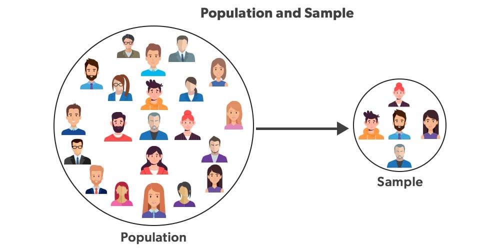
Population vs. Sample

• Population: The entire group that is the subject of the study.

  • Example: All 7,000 students at AUC
  • Notation: \(N\) for size, \(\mu\) for mean, \(\sigma\) for standard deviation

• Sample: A subset of the population used for making inferences about the population.

  • Example: A survey of 100 AUC students
  • Notation: \(n\) for size, \(\bar{x}\) for mean, \(s\) for standard deviation

Methods of Collecting Data

• Surveys: Questionnaires or interviews.
• Observations: Systematic observation and recording.
• Experiments: Controlled settings to observe effects.
• Archival Data: Existing records and databases.

Types of Variables

• Quantitative Variables: Numeric data that can be measured.

  • Continuous: Can take any value within a range (e.g., GPA).
  • Discrete: Specific, countable values (e.g., Number of Courses).

• Qualitative Variables: Descriptive, non-numeric data.

• Nominal: Categories without order (e.g., Majors).

• Ordinal: Categories with order but not equally spaced (e.g., Class Standing: Freshman, Sophomore, etc.).

Measures of Central Tendency 1/3

• Mean: The average of all data points.

  • Population Mean: \(\mu = \frac{\sum_{i=1}^{N} x_i}{N}\)

    • Example: Average GPA of all 7,000 AUC students is \(\mu = 3.5\)

  • Sample Mean: \(\bar{x} = \frac{\sum_{i=1}^{n} x_i}{n}\)

    • Example: Average GPA of a sampled 100 AUC students is \(\bar{x} = 3.48\)

Measures of Central Tendency 2/3

• Median: Middle value when data is sorted

  • Steps to find Median:

    • Sort the data in ascending order

      • If \(n\) is odd, the median is the value at \(\frac{n+1} 2\)th position
      • If \(n\) is even, the median is the average of values at \(\frac{n} 2\) and \(\frac{n} 2 + 1\) positions

• Mode: The most frequently occurring value.

Measures of Central Tendency 3/3

When to use each measure

• Use the mean for normally distributed data
• Use the median when the data is skewed or has outliers
• Use the mode when dealing with categorical data

Measures of Dispersion 1/2

• Range: Difference between the highest and lowest values.

  • Example: highest GPA: \(4.0\), lowest GPA: \(2.9\)

    • Range: \(4.0−2.9=1.1\)

• Variance: Average of the squared differences from the Mean.

  • Population Variance: \(\sigma^2 = \frac{\sum_{i=1}^{N} (x_i - \mu)^2}{N}\)
  • Sample Variance: \(s^2 = \frac{\sum_{i=1}^{n} (x_i - \bar{x})^2}{n-1}\)

• Standard Deviation: Square root of the variance.

  • Population Standard Deviation: \(\sigma = \sqrt{\sigma^2}\)
  • Sample Standard Deviation: \(s = \sqrt{s^2}\)

Measures of Dispersion 2/2

When to use each measure

• The range is great for a quick overview, but it is sensitive to outliers.
• Variance and standard deviation are more robust and provide a clearer picture of the spread in your data.

Setting-up R & RStudio & Google Colab